5 Figure 4
Fig. 4: Identification of two proteomic biomarkers for predicting the outcome of adjuvant chemotherapy in PDAC patients. (a) Scatter plot of the log2 (HR) versus the -log10 (interaction term P-value) of the chemotherapy-by-biomarker interaction term calculated by Cox proportional-hazards models in terms of OS. Notably, the interaction term P-values were not adjusted for multiple hypotheses in this analysis. The blue and red dots represent, respectively, the favorable and unfavorable proteomic biomarkers for adjuvant chemotherapy of PDAC (interaction term P-value < 0.05). The top two proteins are marked with black circle labels. (b) Forest plots of multivariable Cox proportional-hazards regression for NDUFB8 and CEMIP2, respectively. (c-d) Kaplan-Meier survival curves comparing OS between patient subgroups stratified by both adjuvant chemotherapy and high/low abundance (median cutoff) of NDUFB8 (c) and CEMIP2 (d). P-values were calculated using the log-rank test, and the hazard ratios calculated using the univariable Cox regression analysis. (e) GSEA of oxidative phosphorylation and ribosome comparing two patient subgroups stratified by NDUFB8 abundance (left) or comparing PDAC cells between NDUFB8 silencing and control groups (middle and right). RNA and proteins of NDUFB8 were ranked by log2(FC) between two subgroups. Each run was performed with 1,000 permutations. Pathways significantly up-regulated in the NDUFB8-high group (NES > 0, P-value < 0.05, and adjusted P-value < 0.25) were visualized. The dashed line represents P-value of 0.05. (f) GSEA of ECM glycoproteins and epithelial-mesenchymal transition comparing two patient subgroups stratified by CEMIP2 abundance or comparing PDAC cells between CEMIP2 silencing and control groups. RNA and proteins of CEMIP2 were ranked by log2(FC) between two subgroups. Each run was performed with 1,000 permutations. Pathways significantly up regulated in the CEMPI2-high group (NES > 0, P-value < 0.05, and adjusted P-value < 0.25) were visualized. The dashed line represented P-value of 0.05. (g) The levels of hyaluronan in PDO medium, as detected by ELISA. (h) Masson’s Trichrome collagen staining of PDOs. (i-j) IF stainingof -cadherin (i) and Vimentin (j). Cells were stained for markers (orange color) and counterstained with DAPI (blue) to visualize the nuclei.
5.1 (a) Chemotherapy biomarker
Scatter plot of the log2(hazard ratios) versus the -log10(P-values) of the chemotherapy-by-biomarker interaction term calculated by Cox proportional-hazards models in terms of OS. The blue and red dots represent, respectively, the favorable and unfavorable proteomic biomarkers for adjuvant chemotherapy of PDAC (interaction P-value < 0.05). The top two proteins are marked with black circle labels.
library(openxlsx)
library(tidyverse)
library(stringr)
library(survival)
library(survminer)
library(pbapply)
library(ggthemes)
dir.create("./results/Figure4")
#----------------------------------------------------------------------------------
#  Step 1: Load the Data
#----------------------------------------------------------------------------------
deg <- readRDS("./data/proteomics/wgcna/2D-node.data.rds")  # DEG & module genes
pro <- readRDS("./data/proteomics/20230412_PDAC_PRO_exp.rds")
cli <- readRDS("./data/clinical/20230412_PDAC_191_patients_clinical.rds")
#----------------------------------------------------------------------------------
#  Step 2: Coxph data
#----------------------------------------------------------------------------------
# clinical data + DEG genes' expression data
deg <- deg %>% filter(proSig !="zz") %>% pull(Gene) # 1860 DEG genes
rownames(cli) <- cli$ID
id.inter <- intersect(rownames(cli),colnames(pro)) # 191 patients
pro <- pro[deg,id.inter] %>% t()
identical(rownames(cli),rownames(pro))
biomarker_data <- cbind(cli %>% dplyr::select(OS_Time,OS_Status,Censoring_chemo),pro)
# category attribute: chemotherapy treatment
biomarker_data <- biomarker_data %>% mutate(chem=factor(Censoring_chemo,levels = c("0","1")))
#----------------------------------------------------------------------------------
#  Step 3: Coxph
#----------------------------------------------------------------------------------
# Coxph : OS ~ chemotherapy*gene
ls_re <- pbapply::pblapply(colnames(pro),FUN=function(g){
    data <- biomarker_data %>% select(OS_Time,OS_Status,chem) %>%
            mutate(Gene=biomarker_data%>%pull(g))
    fit  <- coxph( Surv(OS_Time,OS_Status) ~ Gene*chem ,data=data) ## interaction term
    broom::tidy(fit) %>% mutate(HR=exp(estimate)) %>% select(p.value,HR) %>% t() %>% as.vector()
})
# result
res <- do.call(rbind,ls_re)
colnames(res) <- c("biomarker_p","biomarker_HR","chemotherapy_p",
                    "chemotherapy_HR","interaction_p","interaction_HR")
## predictive biomarker
res <- res %>% as_tibble() %>% mutate(Gene=colnames(pro)) %>%
            arrange(interaction_p) %>%
            dplyr::select(Gene,everything())
# cutoff
res[which(res$interaction_HR>1 & res$interaction_p <0.05),"group"] = "bad_biomarker"
res[which(res$interaction_HR<1 & res$interaction_p <0.05),"group"] = "good_biomarker"
table(res$group)
#----------------------------------------------------------------------------------
#  Step 4: Visualization
#----------------------------------------------------------------------------------
color.tri <- c("#D01910","#00599F","#444444")  # up ,down ,not
## volcano
res <- res %>% mutate(group=factor(group,levels = c("bad_biomarker","good_biomarker")),
                      Label=Gene,
                      Label=replace(Label,is.na(group),""))
res <- res %>% mutate(log2HR=log2(interaction_HR)) %>%
        mutate(logP= -log10(interaction_p))
p <- ggscatter(res,
               x = "log2HR", y = "logP",
               color = "group", size = 1,
               main = paste0("Predictive biomarker for chemotherapy"),
               xlab = "log2(HR)", ylab = "-log10(Pvalue)",
               palette = color.tri,
               label = res$Label,font.label = 6, , repel = T)+
               theme_base()+
               geom_hline(yintercept = -log10(0.05), linetype="dashed", color = "#222222") +
      theme(plot.background = element_blank())
ggsave("./results/Figure4/4A-Predictive-biomarker.pdf", p, width = 10, height = 8)
write.xlsx(as.data.frame(res),"./results/Figure4/4A-Predictive-biomarker.xlsx",colNames=T,rowNames=F,overwrite = T)
5.2 (b) Forest plots of multivariable Cox
Forest plots of multivariable Cox proportional-hazards regression for NDUFB8 and CEMIP2, respectively.
library(forestmodel)
library(RColorBrewer)
#----------------------------------------------------------------------------------
#  Step 1: Load the Data
#----------------------------------------------------------------------------------
# Sample information and clinical characteristics of the 191 PDAC patients (the RJ-cohort 1)
rj1 <- read.xlsx("./data/Extended Data Table 2.xlsx", startRow = 2)
rj1$`LassoLevel (High vs. Low)` <- ifelse(rj1$LassoLevel == 'High', 1, 0)
rj1$`Adjuvant_therapy (Yes vs. No)` <- ifelse(rj1$Censoring_chemo == 'Chem', 1, 0)
rj1$`Stage (III vs. I_II)` <- ifelse(rj1$Stage == 'III', 1, 0)
rj1$`NDUFB8 (High vs. Low)` <- ifelse(rj1$NDUFB8_l == 'High', 1, 0)
rj1$`CEMIP2 (High vs. Low)` <- ifelse(rj1$CEMIP2_l == 'High', 1, 0)
rj1$`Sex (Male vs. Female)` <- ifelse(rj1$Gender == 'Male', 1, 0)
rj1$`Margin (R1 vs. R0)` <- ifelse(rj1$Margin == 'R1', 1, 0)
rj1$`Smoking (Yes vs. No)` <- rj1$Smoking
rj1$`Drinking (Yes vs. No)` <- rj1$Drinking
#----------------------------------------------------------------------------------
#  Step 2: plot for NDUFB8 * Adjuvant_therapy
#----------------------------------------------------------------------------------
# custom panels for column: Adjust the font style, thickness, and column width of variables in the graph
forest.panels <- list(
  list(width = 0.01),
  list(width = 0.1, display = ~variable,
       fontface = "bold", heading = "Variable"),
  list(width = 0.1, display = ~level),
  list(width = 0.05, display = ~n, hjust = 1, heading = "N"),
  list(width = 0.03, item = "vline", hjust = 0.5),
  list(width = 0.55, item = "forest", hjust = 0.5,
       heading = "Hazard ratio", linetype = "dashed",line_x = 0),
  list(width = 0.03, item = "vline", hjust = 0.5),
  list(width = 0.12, display = ~ ifelse(reference, "Reference", sprintf("%0.3f (%0.3f, %0.3f)",
                                                                        trans(estimate), trans(conf.low), trans(conf.high))), display_na = NA),
  list(width = 0.03,
       display = ~ ifelse(reference, "", format.pval(p.value, digits = 1, eps = 0.001) ),
       display_na = NA, hjust = 1, heading = "p"),
  list(width = 0.03))

Interaction <- rj1[["NDUFB8"]] * rj1[['Adjuvant_therapy (Yes vs. No)']]

pdf('./results/Figure4/Figure4b-1.pdf', width = 10, height = 6)
print(forest_model(coxph(as.formula(paste0('Surv(OS_month, OS_status) ~', '`', "NDUFB8", '`', '+ `Adjuvant_therapy (Yes vs. No)` + Interaction + Age + `Sex (Male vs. Female)` + `Stage (III vs. I_II)` + `Margin (R1 vs. R0)` + CA19_9 + `Smoking (Yes vs. No)` + `Drinking (Yes vs. No)`')), data = rj1), panels = forest.panels, factor_separate_line = F))
dev.off()
#----------------------------------------------------------------------------------
#  Step 3: plot for CEMIP2 * Adjuvant_therapy
#----------------------------------------------------------------------------------
Interaction <- rj1[["CEMIP2"]] * rj1[['Adjuvant_therapy (Yes vs. No)']]
pdf('./results/Figure4/Figure4b-2.pdf', width = 10, height = 6)
print(forest_model(coxph(as.formula(paste0('Surv(OS_month, OS_status) ~', '`', "CEMIP2", '`', '+ `Adjuvant_therapy (Yes vs. No)` + Interaction + Age + `Sex (Male vs. Female)` + `Stage (III vs. I_II)` + `Margin (R1 vs. R0)` + CA19_9 + `Smoking (Yes vs. No)` + `Drinking (Yes vs. No)`')), data = rj1), panels = forest.panels, factor_separate_line = F))
dev.off()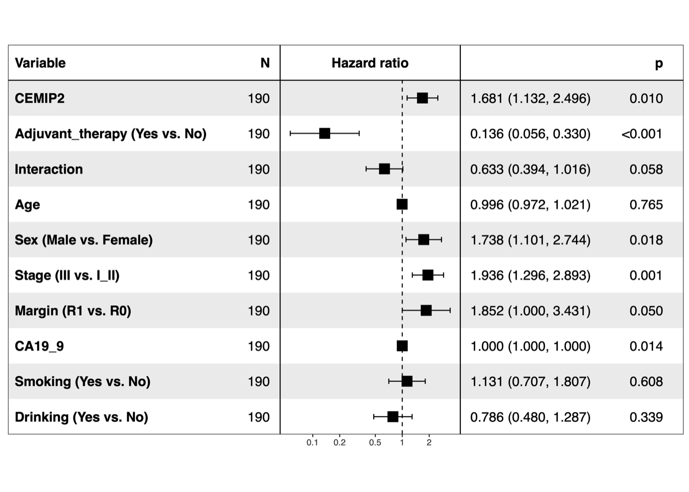
5.3 (cd) Kaplan-Meier curves of NDUFB8/CEMIP2
Kaplan-Meier curves comparing OS between patient subgroups stratified by both adjuvant chemotherapy and high/low abundance (median cutoff) of NDUFB8 (c) and CEMIP2 (d). P-values were calculated using the log-rank test, and the hazard ratios calculated using the univariable Cox regression analysis.
#----------------------------------------------------------------------------------
#  Step 1: Load the data
#----------------------------------------------------------------------------------
# (1) Sample information and clinical characteristics of the 191 PDAC patients (the RJ-cohort 1)
rj1.cohort <- read.xlsx("./data/Extended Data Table 2.xlsx", startRow = 2)
#           ID     Proteomic_ID        RNAseq_ID Age Gender      BMI DM Smoking
# 1 RJ-01-0020 RJ-01-0020-T_PRO RJ-01-0020-T_RNA  61 Female 19.63000  1       0
# 2 RJ-01-0038 RJ-01-0038-T_PRO RJ-01-0038-T_RNA  73   Male 22.46003  0       0
# 3 RJ-01-0050 RJ-01-0050-T_PRO RJ-01-0050-T_RNA  69 Female 17.63085  0       0
# 4 RJ-01-0069 RJ-01-0069-T_PRO RJ-01-0069-T_RNA  69 Female 17.48179  1       0
# 5 RJ-01-0070 RJ-01-0070-T_PRO RJ-01-0070-T_RNA  65   Male 23.43750  0       0
# 6 RJ-01-0074 RJ-01-0074-T_PRO RJ-01-0074-T_RNA  61   Male 23.66144  0       0

plot.cohort <- rj1.cohort %>%
                    mutate(Censoring_chemo_rev = Censoring_chemo,
                           Censoring_chemo = factor(as.character(Censoring_chemo), levels = c("Chem","NoChem")),
                           Censoring_chemo_rev = factor(as.character(Censoring_chemo_rev), levels = c("NoChem","Chem"))) %>%
                    mutate(NDUFB8_l = factor(as.character(NDUFB8_l), levels = c("Low","High")),
                           CEMIP2_l = factor(as.character(CEMIP2_l), levels = c("Low","High"))) %>%
                    mutate(GemType_rev = GemType,
                           GemType = factor(as.character(GemType), levels = c("Gem","NonGem","NoChem")),
                           GemType_rev = factor(as.character(GemType_rev), levels = c("NoChem","Gem","NonGem")))

summary(coxph(Surv(OS_month, OS_status) ~ Censoring_chemo_rev * NDUFB8, data = plot.cohort))
summary(coxph(Surv(OS_month, OS_status) ~ Censoring_chemo_rev * CEMIP2, data = plot.cohort))
#----------------------------------------------------------------------------------
#  Step 2: OS survival stratified by lasso level in [NDUFB8 low] patients
#----------------------------------------------------------------------------------
plot.data <- plot.cohort[which(plot.cohort$NDUFB8_l == "Low"), ]
info <- summary(coxph(Surv(OS_month, OS_status) ~ Censoring_chemo_rev, data = plot.data))
anno.text <- ""
for (i in 1:nrow(info$conf.int)) {
  anno.text <- paste0(anno.text, "\n", paste0(rownames(info$conf.int)[i], " HR=", round(info$conf.int[i, 1], 3), " CI=", round(info$conf.int[i, 3], 3), "-", round(info$conf.int[i, 4], 3), " P=", signif(info$coefficients[i, 5], 4) ))
}
anno.text <- paste0(anno.text, "\nKaplan-Meier P=", signif(survdiff(Surv(OS_month, OS_status) ~ Censoring_chemo_rev, data = plot.data)$pvalue, 4) )
anno.text <- str_replace_all(anno.text, "Censoring_chemo_rev", "")
fit <- survfit(Surv(OS_month, OS_status) ~ Censoring_chemo, data = plot.data)
p1 <- ggsurvplot(fit,
                 data = plot.data,
                 xlab = 'Time (Months)',
                 pval = TRUE,
                 risk.table = TRUE,
                 risk.table.height = 0.28,
                 legend.labs = c("Chem","NoChem"),
                 conf.int = TRUE, conf.int.alpha = 0.05,
                 palette = c("#00599F","#d80700"),
                 axes.offset = TRUE,
                 break.time.by = 12,  xlim = c(0, 48),
                 title= paste0("OS NDUFB8_low Censoring_chemo \n", anno.text))
#----------------------------------------------------------------------------------
#  Step 3: OS survival stratified by lasso level in [NDUFB8 High] patients
#----------------------------------------------------------------------------------
plot.data <- plot.cohort[which(plot.cohort$NDUFB8_l == "High"), ]
info <- summary(coxph(Surv(OS_month, OS_status) ~ Censoring_chemo_rev, data = plot.data))
anno.text <- ""
for (i in 1:nrow(info$conf.int)) {
  anno.text <- paste0(anno.text, "\n", paste0(rownames(info$conf.int)[i], " HR=", round(info$conf.int[i, 1], 3), " CI=", round(info$conf.int[i, 3], 3), "-", round(info$conf.int[i, 4], 3), " P=", signif(info$coefficients[i, 5], 4) ))
}
anno.text <- paste0(anno.text, "\nKaplan-Meier P=", signif(survdiff(Surv(OS_month, OS_status) ~ Censoring_chemo_rev, data = plot.data)$pvalue, 4) )
anno.text <- str_replace_all(anno.text, "Censoring_chemo_rev", "")
fit <- survfit(Surv(OS_month, OS_status) ~ Censoring_chemo, data = plot.data)
p2 <- ggsurvplot(fit,
                 data = plot.data,
                 xlab = 'Time (Months)',
                 pval = TRUE,
                 risk.table = TRUE,
                 risk.table.height = 0.28,
                 legend.labs = c("Chem","NoChem"),
                 conf.int = TRUE, conf.int.alpha = 0.05,
                 palette = c("#00599F","#d80700"),
                 axes.offset = TRUE,
                 break.time.by = 12,  xlim = c(0, 48),
                 title= paste0("OS NDUFB8_high Censoring_chemo \n", anno.text))
#----------------------------------------------------------------------------------
#  Step 4: OS survival stratified by lasso level in [CEMIP2 low] patients
#----------------------------------------------------------------------------------
plot.data <- plot.cohort[which(plot.cohort$CEMIP2_l == "Low"), ]
info <- summary(coxph(Surv(OS_month, OS_status) ~ Censoring_chemo_rev, data = plot.data))
anno.text <- ""
for (i in 1:nrow(info$conf.int)) {
  anno.text <- paste0(anno.text, "\n", paste0(rownames(info$conf.int)[i], " HR=", round(info$conf.int[i, 1], 3), " CI=", round(info$conf.int[i, 3], 3), "-", round(info$conf.int[i, 4], 3), " P=", signif(info$coefficients[i, 5], 4) ))
}
anno.text <- paste0(anno.text, "\nKaplan-Meier P=", signif(survdiff(Surv(OS_month, OS_status) ~ Censoring_chemo_rev, data = plot.data)$pvalue, 4) )
anno.text <- str_replace_all(anno.text, "Censoring_chemo_rev", "")
fit <- survfit(Surv(OS_month, OS_status) ~ Censoring_chemo, data = plot.data)
p3 <- ggsurvplot(fit,
                 data = plot.data,
                 xlab = 'Time (Months)',
                 pval = TRUE,
                 risk.table = TRUE,
                 risk.table.height = 0.28,
                 legend.labs = c("Chem","NoChem"),
                 conf.int = TRUE, conf.int.alpha = 0.05,
                 palette = c("#00599F","#d80700"),
                 axes.offset = TRUE,
                 break.time.by = 12,  xlim = c(0, 48),
                 title= paste0("OS CEMIP2_low Censoring_chemo \n", anno.text))
#----------------------------------------------------------------------------------
#  Step 5: OS survival stratified by lasso level in [CEMIP2 High] patients
#----------------------------------------------------------------------------------
plot.data <- plot.cohort[which(plot.cohort$CEMIP2_l == "High"), ]
info <- summary(coxph(Surv(OS_month, OS_status) ~ Censoring_chemo_rev, data = plot.data))
anno.text <- ""
for (i in 1:nrow(info$conf.int)) {
  anno.text <- paste0(anno.text, "\n", paste0(rownames(info$conf.int)[i], " HR=", round(info$conf.int[i, 1], 3), " CI=", round(info$conf.int[i, 3], 3), "-", round(info$conf.int[i, 4], 3), " P=", signif(info$coefficients[i, 5], 4) ))
}
anno.text <- paste0(anno.text, "\nKaplan-Meier P=", signif(survdiff(Surv(OS_month, OS_status) ~ Censoring_chemo_rev, data = plot.data)$pvalue, 4) )
anno.text <- str_replace_all(anno.text, "Censoring_chemo_rev", "")
fit <- survfit(Surv(OS_month, OS_status) ~ Censoring_chemo, data = plot.data)
p4 <- ggsurvplot(fit,
                 data = plot.data,
                 xlab = 'Time (Months)',
                 pval = TRUE,
                 risk.table = TRUE,
                 risk.table.height = 0.28,
                 legend.labs = c("Chem","NoChem"),
                 conf.int = TRUE, conf.int.alpha = 0.05,
                 palette = c("#00599F","#d80700"),
                 axes.offset = TRUE,
                 break.time.by = 12,  xlim = c(0, 48),
                 title= paste0("OS CEMIP2_high Censoring_chemo \n", anno.text))
# output
p <- arrange_ggsurvplots(list(p1, p2, p3, p4), ncol = 4, nrow = 1, print = FALSE)
ggsave(paste0("./results/Figure4/Figure4cd.pdf"), p, width = 20, height = 8)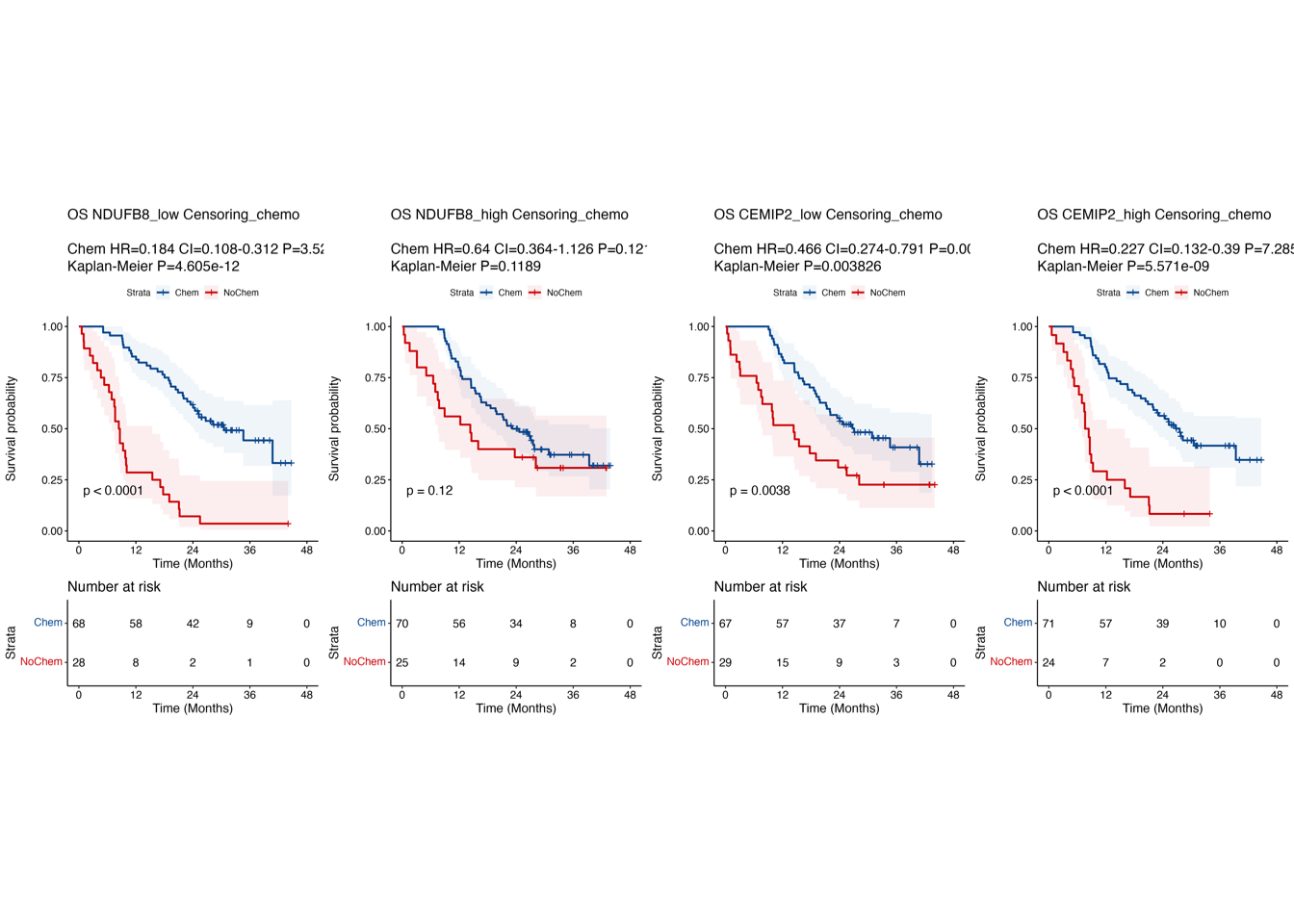
5.4 (e) GSEA stratified by NDUFB8
GSEA of oxidative phosphorylation and ribosome comparing two patient subgroups stratified by NDUFB8 abundance (left) or comparing PDAC cells between NDUFB8 silencing and control groups (middle and right). RNA and proteins of NDUFB8 were ranked by log2(FC) between two subgroups. Each run was performed with 1,000 permutations. Pathways significantly up-regulated in NDUFB8-high group (NES > 0, P-value < 0.05 and adjusted P-value < 0.05) were visualized. The dashed line represented P-value = 0.05.
#----------------------------------------------------------------------------------
#  Step 1: Load the data
#----------------------------------------------------------------------------------
# enrichment results
plot.data.1 <- read.xlsx("./data/Figure4/1.protein.deg.NH_NL.GSEA_1k.xlsx")
plot.data.2 <- read.xlsx("./data/Figure4/1.CFPAC.deg.NH_NL.GSEA_1k.xlsx")
plot.data.3 <- read.xlsx("./data/Figure4/1.8988.deg.NH_NL.GSEA_1k.xlsx")
#                                 ID                      Description setSize enrichmentScore
# 1                    KEGG_RIBOSOME                    KEGG_RIBOSOME      87       0.6233584
# 2                 KEGG_SPLICEOSOME                 KEGG_SPLICEOSOME     126       0.4505875
# 3          HALLMARK_MYC_TARGETS_V1          HALLMARK_MYC_TARGETS_V1     199       0.3968739
# 4 HALLMARK_TNFA_SIGNALING_VIA_NFKB HALLMARK_TNFA_SIGNALING_VIA_NFKB     199      -0.3993534
# 5   HALLMARK_INFLAMMATORY_RESPONSE   HALLMARK_INFLAMMATORY_RESPONSE     200      -0.3683088
# 6  KEGG_HEMATOPOIETIC_CELL_LINEAGE  KEGG_HEMATOPOIETIC_CELL_LINEAGE      85      -0.3989387
plot.data.1$Omics <- "Protein"
plot.data.2$Omics <- "CFPAC"
plot.data.3$Omics <- "8988"
plot.data <- rbind(plot.data.1, plot.data.2, plot.data.3) %>%
                      mutate(SignP= -log10(pvalue))
plot.data$SignP[which(plot.data$NES < 0)] <- plot.data$SignP[which(plot.data$NES < 0)] * -1
plot.pathway <- c("KEGG_RIBOSOME","KEGG_OXIDATIVE_PHOSPHORYLATION")
plot.data.sub <- plot.data[plot.data$ID %in% plot.pathway, ]
plot.data.sub$Omics <- factor(as.character(plot.data.sub$Omics), levels = c("Protein","CFPAC","8988"))
#----------------------------------------------------------------------------------
#  Step 2: plot
#----------------------------------------------------------------------------------
p <- ggbarplot(plot.data.sub, x = "ID", y = "SignP",
               color = "#FFC25F", fill = "#FFC25F",
               position = position_dodge(0.8),
               order = rev(plot.pathway),
               main = "GSEA NDUFB8 high vs low")
p <- p + geom_hline(yintercept = c(1.30), linetype="dashed", color = "#222222")
p <- p + facet_wrap(~ Omics, ncol = 3)
p <- p + scale_y_continuous(limits = c(0, 3.5), expand = c(0,0))
p <- p + coord_flip() + theme_base()
ggsave(paste0("./results/Figure4/Figure4e.pdf"), p, width = 13, height = 3)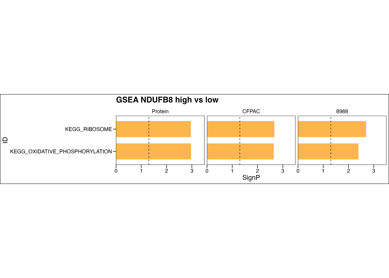
5.5 (f) GSEA stratified by CEMIP2
GSEA of ECM glycoproteins and epithelial-mesenchymal transition comparing two patient subgroups stratified by CEMIP2 abundance or comparing PDAC cells between CEMIP2 silencing and control groups. RNA and proteins of CEMIP2 were ranked by log2(FC) between two subgroups. Each run was performed with 1,000 permutations. Pathways significantly up-regualted in CEMPI2-high group (NES > 0, P-value < 0.05 and adjusted P-value < 0.05) were visualized. The dashed line represented P-value = 0.05.
#----------------------------------------------------------------------------------
#  Step 1: Load the data
#----------------------------------------------------------------------------------
# enrichment results
plot.data.1 <- read.xlsx("./data/Figure4/2.protein.deg.CH_CL.GSEA_1k.xlsx")
plot.data.2 <- read.xlsx("./data/Figure4/2.CFPAC.deg.CH_CL.GSEA_1k.xlsx")
plot.data.3 <- read.xlsx("./data/Figure4/2.8988.deg.CH_CL.GSEA_1k.xlsx")
#                                           ID                                Description setSize
# 1           HALLMARK_TNFA_SIGNALING_VIA_NFKB           HALLMARK_TNFA_SIGNALING_VIA_NFKB     199
# 2                              KEGG_RIBOSOME                              KEGG_RIBOSOME      87
# 3                           HALLMARK_HYPOXIA                           HALLMARK_HYPOXIA     200
# 4 HALLMARK_EPITHELIAL_MESENCHYMAL_TRANSITION HALLMARK_EPITHELIAL_MESENCHYMAL_TRANSITION     197
# 5                       HALLMARK_COAGULATION                       HALLMARK_COAGULATION     138
# 6                 HALLMARK_KRAS_SIGNALING_UP                 HALLMARK_KRAS_SIGNALING_UP     200
plot.data.1$Omics <- "Protein"
plot.data.2$Omics <- "CFPAC"
plot.data.3$Omics <- "8988"
plot.data <- rbind(plot.data.1, plot.data.2, plot.data.3)
plot.data$SignP <- -log10(plot.data$pvalue)
plot.data$SignP[which(plot.data$NES < 0)] <- plot.data$SignP[which(plot.data$NES < 0)] * -1
plot.pathway <- c("NABA_ECM_GLYCOPROTEINS", "HALLMARK_EPITHELIAL_MESENCHYMAL_TRANSITION")
plot.data.sub <- plot.data[plot.data$ID %in% plot.pathway, ]
plot.data.sub$Omics <- factor(as.character(plot.data.sub$Omics), levels = c("Protein","CFPAC","8988"))
#----------------------------------------------------------------------------------
#  Step 2: plot
#----------------------------------------------------------------------------------
p <- ggbarplot(plot.data.sub, x = "ID", y = "SignP",
               color = "#FFC2C1", fill = "#FFC2C1",
               position = position_dodge(0.8),
               order = rev(plot.pathway),
               main = "GSEA CEMIP2 high vs low")
p <- p + geom_hline(yintercept = c(1.30), linetype="dashed", color = "#222222")
p <- p + facet_wrap(~ Omics, ncol = 3)
p <- p + scale_y_continuous(limits = c(0, 3.5), expand = c(0,0))
p <- p + coord_flip() + theme_base()
ggsave(paste0("./results/Figure4/Figure4f.pdf"), p, width = 13, height = 3)