3 Figure 2
Fig. 2: Proteomic landscape for PDACs and clinical relevance of functional protein modules (a) WGCNA identifies 32 functional protein modules (ME01-32) enriched in proteomic data for tumor samples. Each network node represents one protein, color-coded by the different functional modules. (b) Overlay of the significantly up/down-regulated proteins between tumors and TACs onto the network nodes. (c) Bar plot showing the normalized enrichment score of the 32 protein modules in tumors and TACs using the data from RJ-cohort 1 as well as the Cao et al cohort. P-values were calculated using the Mann-Whitney U test and adjusted using the BH method. An adjusted P-value < 0.05 was labelled in red color. (d) Association of the enrichment score of the 32 modules with clinical data. Detailed information regarding the correlation analysis between module scores and clinical data can be found in Extended Data Table 3 and the Methods section. (e) Kaplan-Meier survival curves comparing OS between patient subgroups stratified by both adjuvant therapy and the high/low abundance (median cutoff) of ME11. P-values were calculated using the log-rank test, and the hazard ratios calculated using the univariable Cox regression analysis.
3.1 (a) WGCNA
We performed weighted correlation network analysis WGCNA on proteomic data from tumor samples, identifying a total of 32 functional modules.
library(WGCNA)
dir.create("./results/Figure2/WGCNA",recursive = T)
#----------------------------------------------------------------------------------
#  Step 1: Loading expression data and set parameters
#----------------------------------------------------------------------------------
protein.nona.tumor <- readRDS("./data/proteomics/wgcna/20230412_PDAC_PRO_Tumor_exp.rds")
corType = "pearson"
corFnc = ifelse(corType=="spearman", cor, bicor)
maxPOutliers = ifelse(corType=="pearson",1, 0.05)
# input data normalization
plot.mat <- t(protein.nona.tumor - rowMeans(protein.nona.tumor)) # row: samples | col: genes
#----------------------------------------------------------------------------------
#  Step 2: identification of outlier samples
#----------------------------------------------------------------------------------
sampleTree = hclust(dist(plot.mat), method = "ward.D")
pdf(paste0("./results/Figure2/WGCNA/1.tree.pdf"), width = 20, height = 9)
plot(sampleTree, main = "Sample clustering to detect outliers", sub="", xlab="")
dev.off()
#----------------------------------------------------------------------------------
#  Step 3: analysis of network topology
#----------------------------------------------------------------------------------
# Choose a set of soft-thresholding powers
powers = c(c(1:10), seq(from = 12, to = 30, by = 2))
# Call the network topology analysis function
sft = pickSoftThreshold(plot.mat, powerVector=powers,
                        networkType="unsigned", verbose=5)
# Plot the results:
pdf(paste0("./results/Figure2/WGCNA/2.power.pdf"), width = 12, height = 8)
par(mfrow = c(1,2))
cex1 = 0.9
plot(sft$fitIndices[,1], -sign(sft$fitIndices[,3])*sft$fitIndices[,2],
     xlab="Soft Threshold (power)",
     ylab="Scale Free Topology Model Fit, signed R^2",type="n",
     main = paste("Scale independence"))
text(sft$fitIndices[,1], -sign(sft$fitIndices[,3])*sft$fitIndices[,2],
     labels=powers,cex=cex1,col="red")
abline(h=0.85,col="red")
plot(sft$fitIndices[,1], sft$fitIndices[,5],
     xlab="Soft Threshold (power)",ylab="Mean Connectivity", type="n",
     main = paste("Mean connectivity"))
text(sft$fitIndices[,1], sft$fitIndices[,5], labels=powers,
     cex=cex1, col="red")
dev.off()
#----------------------------------------------------------------------------------
#  Step 4: soft threshold : power
#----------------------------------------------------------------------------------
power = sft$powerEstimate
power
#----------------------------------------------------------------------------------
#  Step 5: One-step network construction and module detection
#----------------------------------------------------------------------------------
net = blockwiseModules(plot.mat, power = power, maxBlockSize = ncol(plot.mat),
                       TOMType = "signed", minModuleSize = 20,
                       reassignThreshold = 0, mergeCutHeight = 0.0001,
                       numericLabels = TRUE, pamRespectsDendro = FALSE,
                       saveTOMs=TRUE, corType = corType,
                       maxPOutliers = 1, loadTOMs=TRUE,
                       randomSeed = 931, # seed
                       saveTOMFileBase = paste0("./results/Figure2/WGCNA/WGCNA.tom"),
                       verbose = 3, pearsonFallback = "none", deepSplit = 3 )
# module:
table(net$colors) # 0 corresponds to unclassified genes
# Convert [number] labels to [colors] for plotting
moduleLabels = net$colors
moduleColors = labels2colors(moduleLabels)
# plot
pdf(paste0( "./results/Figure2/WGCNA/3.module.pdf"), width = 8, height = 6)
plotDendroAndColors(net$dendrograms[[1]], moduleColors[net$blockGenes[[1]]],
                    "Module colors",
                    dendroLabels = FALSE, hang = 0.03,
                    addGuide = TRUE, guideHang = 0.05)
dev.off()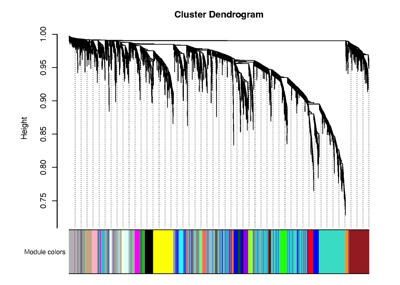
#----------------------------------------------------------------------------------
#  Step 6: Vasualization
#----------------------------------------------------------------------------------
## data
node.data <- readRDS("./data/proteomics/wgcna/2D-node.data.rds")
edge.data <- readRDS("./data/proteomics/wgcna/2D-edge.data.rds")
color.module <- c("#CCCCCC","#ecb888","#af88bb","#a032cb","#efbed6","#fc496a","#b6d37f","#589336","#7fd68e","#52c465","#3372e0","#84d7f6","#5394c3","#6376b3","#7f6cd7","#c4ceff","#fc9d40","#5c95e0","#cd7560","#ff70e4", "#ff8738", "#ffcead","#1cbf8b", "#b76d38", "#1584ff", "#7f006d", "#ffd35f","#E66F73","#F57F20","#1DBB95","#9CB79F","#F0B8D2","#A0485E","#A0688E","#C7E1DF","#51B1DF","#6D97D7","#5D6193","#CEC3E0","#A9917E","#7C7D80","#F4E192","#ADD666")
names(color.module) <- paste0("ME", seq(0,length(color.module)-1) %>% str_pad(width = 2,side = "left",pad = "0"))
## plot network
gg <- ggplot()
gg <- gg + geom_segment(mapping = aes(x = from.x, y = from.y, xend = to.x, yend = to.y),
                        color = "#CCCCCC", size = 0.01, data = edge.data) # draw a straight line
gg <- gg + geom_point(mapping = aes(x = pos.x, y = pos.y, color = Module),
                      size = 2, data = node.data) # add point
gg <- gg + scale_size(range = c(0, 6) * 2) # specifies the minimum and maximum size
gg <- gg + theme_void()
gg <- gg + labs(x = "", y = "", title = paste0("PPI"))
gg <- gg + scale_colour_manual(values = color.module)
ggsave(paste0("./results/Figure2/2A-PRO-modules.png"), gg, width = 10, height = 8)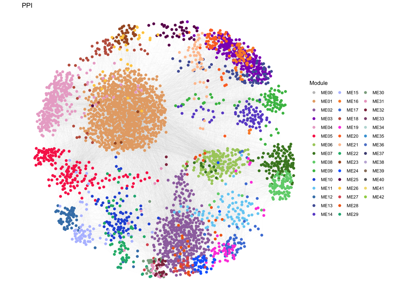
3.2 (b) Significantly up/down-regulated proteins
Overlay of the significantly up/down-regulated proteins between tumors and TACs onto the network nodes. The proteins significantly up- or down-regulated within these modules, when comparing tumors and TACs are depicted in Fig.2b.
#----------------------------------------------------------------------------------------------
#  Overlay the log2 fold change between tumor and TAC on PRO in the WGCNA network
#----------------------------------------------------------------------------------------------
## data
node.data <- readRDS("./data/proteomics/wgcna/2D-node.data.rds") # DEG & module genes
edge.data <- readRDS("./data/proteomics/wgcna/2D-edge.data.rds")
## plot
gg <- ggplot()
gg <- gg + geom_segment(mapping = aes(x = from.x, y = from.y, xend = to.x, yend = to.y),
                        color = "#CCCCCC", size = 0.01, data = edge.data)
gg <- gg + geom_point(mapping = aes(x = pos.x, y = pos.y, color = proSig), size = 1,
                      data = node.data[which(node.data$proSig == "zz"), ])
gg <- gg + geom_point(mapping = aes(x = pos.x, y = pos.y, color = proSig), size = 2.5,
                      data = node.data[which(node.data$proSig != "zz"), ])
gg <- gg + scale_size(range = c(0, 6) * 2)
gg <- gg + theme_void()
gg <- gg + labs(x = "", y = "", title = paste0("color by proSig"))
gg <- gg + scale_colour_manual(values = c("#00599F","#D01910","#AAAAAA"))
ggsave(paste0("./results/Figure2/2B-proSig.png"), gg, width = 8.5, height = 8)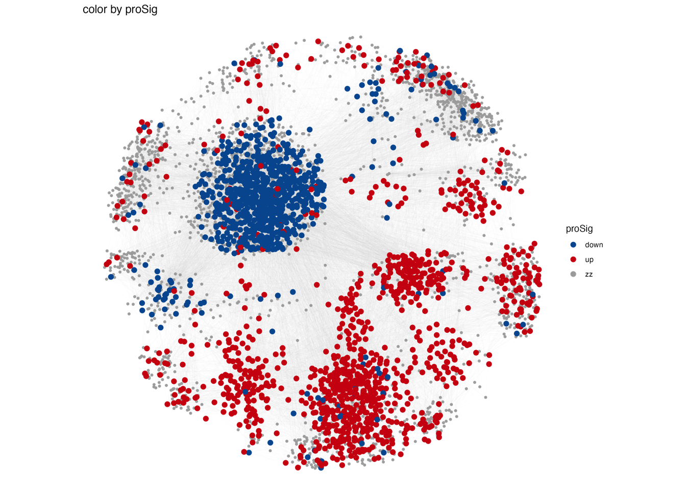
3.3 (c) Modules enrichment score
Bar plot showing the normalized enrichment score of the 32 protein modules in tumors and TACs using the data of our cohort as well as Cao et al cohort.
color.bin <- c("#00599F","#d80700")
#----------------------------------------------------------------------------------
#  Step 1: Load the RJ-cohort 1 Data
#----------------------------------------------------------------------------------
# Scores of the 32 modules in TACs and PDACs of RJ-cohort 1
plot.data <- read.xlsx("./data/Extended Data Table 4.xlsx", sheet = 2, startRow = 2, rowNames = T)
#                       ME01         ME02        ME03       ME04
# RJ-01-0143-N_PRO 0.3474261 -0.114677437 -0.04291552 0.06708347
# RJ-01-0768-N_PRO 0.2532539  0.009051615 -0.03585508 0.03486392
# RJ-01-0697-N_PRO 0.2839048 -0.032966990 -0.02943711 0.05803330
# RJ-01-0609-N_PRO 0.3206755 -0.087559353 -0.05749618 0.10310726
plot.info <- NULL
module.name <- colnames(plot.data)
plot.stat <- data.frame(Module = module.name,
                        Wilcox.P = NA,
                        Wilcox.Padj = NA)
#----------------------------------------------------------------------------------
#  Step 2: wilcox.test
#----------------------------------------------------------------------------------
for (i in 1:ncol(plot.data)) {
  sub <- data.frame(Sample = rownames(plot.data),
                    Score = as.numeric(plot.data[, i]),
                    ScoreScale = scale(as.numeric(plot.data[, i])),
                    Module = colnames(plot.data)[i],
                    Type = substr(rownames(plot.data), 12, 16))
  plot.stat$Wilcox.P[i] <- wilcox.test(sub$ScoreScale ~ sub$Type)$p.value
  plot.info <- rbind(plot.info, sub)
}
plot.info <- plot.info %>% mutate(Type=factor(as.character(Type), levels = c("N_PRO","T_PRO")))
plot.stat <- plot.stat %>% mutate(Wilcox.Padj=p.adjust(Wilcox.P, method = "fdr"))
#----------------------------------------------------------------------------------
#  Step 3: plot
#----------------------------------------------------------------------------------
p <- ggbarplot(plot.info, x = "Module", y = "ScoreScale",
               color = "Type", fill = "Type",
               palette = color.bin, width = 0.5, size = 0,
               add = c("mean_se"), add.params = list(width = 0.5),
               order = module.name,
               position = position_dodge(0.6),
               xlab = "", ylab = "Module Score of Protein")
p <- p + theme_base()
p <- p + geom_hline(yintercept = 0, color = "black")
p <- p + theme(axis.text.x = element_text(angle = 90, hjust = 1, vjust = 0.5))
p <- p + stat_compare_means(aes(group = Type, label = ..p.format..), size = 1, method = "wilcox.test", label.y = 1.2)  + theme(plot.background = element_blank())
#----------------------------------------------------------------------------------
#  Step 4: output
#----------------------------------------------------------------------------------
ggsave(paste0("./results/Figure2/Figure2c-1.pdf"), p, width = 12, height = 4)
write.xlsx(plot.stat, paste0("./results/Figure2/Figure2c.padj-1.xlsx"))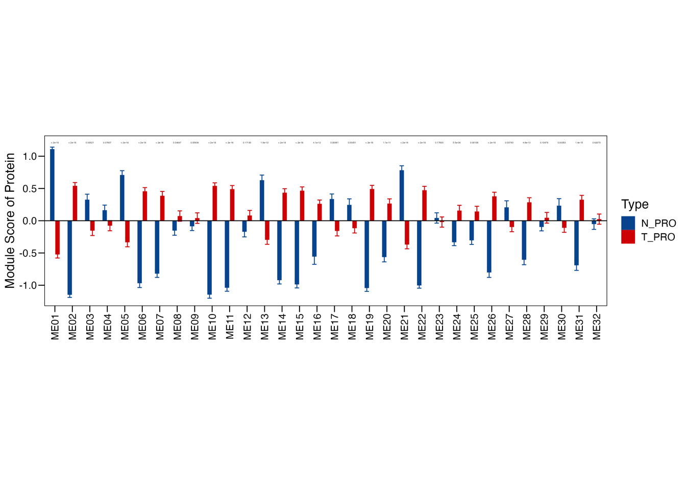
#----------------------------------------------------------------------------------
#  Step 5: Load the Cao et al cohort Data
#----------------------------------------------------------------------------------
module.ssgsea.pro.cell <- readRDS("./data/proteomics/cao.module.ssgsea.pro.rds")
cell.meta.data <- read.xlsx("./data/proteomics/cao.meta.data.xlsx")
cell.all.sample <- c(cell.meta.data$Proteomic_ID, str_replace_all(cell.meta.data$Proteomic_ID, "_T", "_N"))
cell.all.sample <- cell.all.sample[cell.all.sample %in% colnames(module.ssgsea.pro.cell)]
plot.data <- t(module.ssgsea.pro.cell[, cell.all.sample])
plot.info <- NULL
plot.stat <- data.frame(Module = colnames(plot.data),
                        Wilcox.P = NA,
                        Wilcox.Padj = NA)
#----------------------------------------------------------------------------------
#  Step 6: wilcox.test
#----------------------------------------------------------------------------------
for (i in 1:ncol(plot.data)) {
  sub <- data.frame(Sample = rownames(plot.data),
                    Score = as.numeric(plot.data[, i]),
                    ScoreScale = scale(as.numeric(plot.data[, i])),
                    Module = colnames(plot.data)[i],
                    Type = substr(rownames(plot.data), 11, 11))
  plot.stat$Wilcox.P[i] <- wilcox.test(sub$ScoreScale ~ sub$Type)$p.value
  plot.info <- rbind(plot.info, sub)
}
plot.info$Type <- factor(as.character(plot.info$Type), levels = c("N","T"))
plot.stat$Wilcox.Padj <- p.adjust(plot.stat$Wilcox.P, method = "fdr")
#----------------------------------------------------------------------------------
#  Step 7: plot
#----------------------------------------------------------------------------------
p <- ggbarplot(plot.info, x = "Module", y = "ScoreScale",
               color = "Type", fill = "Type",
               palette = color.bin, width = 0.5, size = 0,
               add = c("mean_se"), add.params = list(width = 0.5),
               order = module.name,
               position = position_dodge(0.6),
               xlab = "", ylab = "Module Score of Protein")
p <- p + theme_base()
p <- p + geom_hline(yintercept = 0, color = "black")
p <- p + theme(axis.text.x = element_text(angle = 90, hjust = 1, vjust = 0.5))
p <- p + stat_compare_means(aes(group = Type, label = ..p.format..), size = 1, method = "wilcox.test", label.y = 1.2) + theme(plot.background = element_blank())
#----------------------------------------------------------------------------------
#  Step 8: output
#----------------------------------------------------------------------------------
ggsave(paste0("./results/Figure2/Figure2c-2.pdf"), p, width = 12, height = 4)
write.xlsx(plot.stat, paste0("./results/Figure2/Figure2c.padj-2.xlsx"))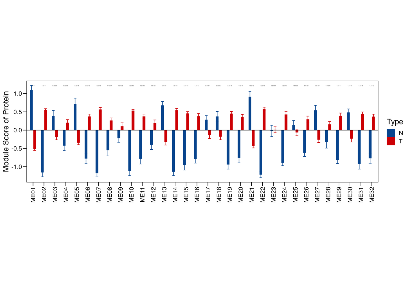
3.4 (d) Association: 32 Module score ~ Clinical trait
Association of the enrichment score of the 32 modules with clinical data and RNA-seq subtype.
library(survival)
#----------------------------------------------------------------------------------
#  Step 1: Loading expression data and set parameters
#----------------------------------------------------------------------------------
# (1) Sample information and clinical characteristics of the 191 PDAC patients (the RJ-cohort 1)
rj1.cohort <- read.xlsx("./data/Extended Data Table 2.xlsx", startRow = 2)
#           ID     Proteomic_ID        RNAseq_ID Age Gender      BMI DM Smoking
# 1 RJ-01-0020 RJ-01-0020-T_PRO RJ-01-0020-T_RNA  61 Female 19.63000  1       0
# 2 RJ-01-0038 RJ-01-0038-T_PRO RJ-01-0038-T_RNA  73   Male 22.46003  0       0
# 3 RJ-01-0050 RJ-01-0050-T_PRO RJ-01-0050-T_RNA  69 Female 17.63085  0       0
# 4 RJ-01-0069 RJ-01-0069-T_PRO RJ-01-0069-T_RNA  69 Female 17.48179  1       0
# 5 RJ-01-0070 RJ-01-0070-T_PRO RJ-01-0070-T_RNA  65   Male 23.43750  0       0
# 6 RJ-01-0074 RJ-01-0074-T_PRO RJ-01-0074-T_RNA  61   Male 23.66144  0       0

# (2) Scores of the 32 modules in TACs and PDACs of RJ-cohort 1.
module.ssgsea.pro.all <- read.xlsx("./data/Extended Data Table 4.xlsx", sheet = 2, startRow = 2, rowNames = T)
module.ssgsea.pro.all <- t(module.ssgsea.pro.all)
#      RJ-01-0143-N_PRO RJ-01-0768-N_PRO RJ-01-0697-N_PRO RJ-01-0609-N_PRO RJ-01-1055-N_PRO
# ME01       0.34742611      0.253253916       0.28390477       0.32067554      0.325797851
# ME02      -0.11467744      0.009051615      -0.03296699      -0.08755935     -0.096947986
# ME03      -0.04291552     -0.035855079      -0.02943711      -0.05749618      0.016639009
# ME04       0.06708347      0.034863920       0.05803330       0.10310726      0.007498371
# ME05       0.19099018      0.100153070       0.14246697       0.16675071      0.127932887
# ME06       0.03893163      0.240865770       0.14178269       0.07618613      0.038306853

# (3) Lasso Score in RJ-cohort 1 RNA-seq
rj1.rnaseq <- read.xlsx("./data/RNA/rj1.rnaseq.lasso.score.xlsx")
#           ID     Proteomic_ID        RNAseq_ID  LassoScore LassoLevel LassoScoreRNA LassoLevelRNA
# 1 RJ-01-0020 RJ-01-0020-T_PRO RJ-01-0020-T_RNA  0.22945083       High     -2.394123          High
# 2 RJ-01-0038 RJ-01-0038-T_PRO RJ-01-0038-T_RNA -0.05725430       High     -2.561299           Low
# 3 RJ-01-0050 RJ-01-0050-T_PRO RJ-01-0050-T_RNA -0.10574547       High     -2.720116           Low
# 4 RJ-01-0069 RJ-01-0069-T_PRO RJ-01-0069-T_RNA -0.69376332        Low     -2.595342           Low
# 5 RJ-01-0070 RJ-01-0070-T_PRO RJ-01-0070-T_RNA -0.03992765       High     -2.581288           Low
# 6 RJ-01-0074 RJ-01-0074-T_PRO RJ-01-0074-T_RNA  0.17797893       High     -2.572467           Low

#----------------------------------------------------------------------------------
#  Step 2: Module score ~ OS/DFS (coxph, prognosis)
#----------------------------------------------------------------------------------
module.name <- rownames(module.ssgsea.pro.all)

plot.info <- NULL
plot.data <- rj1.cohort
plot.info.os <- NULL

## (1) Module score ~ OS
for (i in 1:length(module.name)) {
  # data:  module score -> Low/High level (median cutoff)
  plot.data <- plot.data %>%
              mutate(ME_score = module.ssgsea.pro.all[module.name[i], plot.data$Proteomic_ID] %>% as.numeric()) %>%
              mutate(ME_level=ifelse(ME_score >= median(ME_score),"High","Low")) %>%
              mutate(ME_level=factor(ME_level,levels = c("Low","High")))
  # coxph
  fit <- coxph(Surv(OS_month, OS_status) ~ ME_level, data = plot.data)
  fit.info <- summary(fit)
  fit.p <- survdiff(Surv(OS_month, OS_status) ~ ME_level, data = plot.data)$pvalue
  fit.info.out <- c(module.name[i], "OS", fit.info$conf.int[1, 1], fit.info$coefficients[1,5], "Log-rank test" )
  plot.info.os <- rbind(plot.info.os, fit.info.out)
}
plot.info.os <- as.data.frame(plot.info.os)
colnames(plot.info.os) <- c("Module", "Factor", "Type","P", "Test")
# result
plot.info.os <- plot.info.os %>%
                    mutate(Type=as.numeric(Type),P=as.numeric(P),
                           Padj= p.adjust(P, method = "fdr")) %>%
                    mutate(Tag=case_when(Type>1&P<0.05 ~ "Unfavorable",
                                         Type<1&P<0.05 ~ "Favorable",
                                         .default="notSig" ))
## (1) Module score ~ DFS
plot.data <- rj1.cohort
plot.info.dfs <- NULL
for (i in 1:length(module.name)) {
  # data:  module score -> Low/High level (median cutoff)
  plot.data <- plot.data %>%
              mutate(ME_score = module.ssgsea.pro.all[module.name[i], plot.data$Proteomic_ID] %>% as.numeric()) %>%
              mutate(ME_level=ifelse(ME_score >= median(ME_score),"High","Low")) %>%
              mutate(ME_level=factor(ME_level,levels = c("Low","High")))
  # coxph
  fit <- coxph(Surv(DFS_month, DFS_status) ~ ME_level, data = plot.data)
  fit.info <- summary(fit)
  fit.p <- survdiff(Surv(DFS_month, DFS_status) ~ ME_level, data = plot.data)$pvalue
  fit.info.out <- c(module.name[i], "DFS", fit.info$conf.int[1, 1], fit.info$coefficients[1,5], "Log-rank test" )
  plot.info.dfs <- rbind(plot.info.dfs, fit.info.out)
}
plot.info.dfs <- as.data.frame(plot.info.dfs)
colnames(plot.info.dfs) <- c("Module", "Factor", "Type", "P", "Test")
# result
plot.info.dfs <- plot.info.dfs %>%
                    mutate(Type=as.numeric(Type),P=as.numeric(P),
                           Padj= p.adjust(P, method = "fdr")) %>%
                    mutate(Tag=case_when(Type>1&P<0.05 ~ "Unfavorable",
                                         Type<1&P<0.05 ~ "Favorable",
                                         .default="notSig" ))
#----------------------------------------------------------------------------------
#  Step 3: Module score ~ continuous type clinical trait (cor)
#----------------------------------------------------------------------------------
plot.name <- c("Age","BMI","WBC","Hb","PLT","TBIL","DBIL","ALB","Glu","CA125","CA19_9","CEA","AFP","CA724","Diameter_tumor","Num_Pos_LN","Num_total_LN")
plot.name[! plot.name %in% colnames(rj1.cohort)]
plot.info.cat <- NULL
for (kkk in 1:length(plot.name)) {
  plot.data <- rj1.cohort
  plot.data$Plot <- plot.data[, which(colnames(plot.data) == plot.name[kkk])]
  plot.data <- plot.data[which(!is.na(plot.data$Plot)), ]
  plot.info.cat.sub <- NULL
  for (i in 1:length(module.name)) {
    plot.data$ME_score <- module.ssgsea.pro.all[module.name[i], plot.data$Proteomic_ID] %>% as.numeric()
    sub <- c(module.name[i], plot.name[kkk], cor(plot.data$ME_score, plot.data$Plot, method = "spearman"),
             cor.test(plot.data$ME_score, plot.data$Plot, method = "spearman")$p.value, "Spearman's correlation")
    plot.info.cat.sub <- rbind(plot.info.cat.sub, sub)
  }
  plot.info.cat.sub <- as.data.frame(plot.info.cat.sub)
  colnames(plot.info.cat.sub) <- c("Module", "Factor", "Type","P", "Test")
  plot.info.cat.sub <- plot.info.cat.sub %>%
                            mutate(Type=as.numeric(Type),
                                   P=as.numeric(P),
                                   Padj=p.adjust(P,method="fdr"))
  plot.info.cat <- rbind(plot.info.cat, plot.info.cat.sub)
}
plot.info.cat <- plot.info.cat %>%
                            mutate(Tag=case_when(Type<0&P<0.05 ~ "Negative",
                                                 Type>0&P<0.05 ~ "Positive",
                                                .default="notSig" ))
#----------------------------------------------------------------------------------
#  Step 4: Module score ~ category type clinical trait (Wilcoxon rank-sum test or ANOVA)
#----------------------------------------------------------------------------------
plot.name <- c("Gender","Drinking","Smoking","Ninv","T","N","Stage","Grade")
plot.name[! plot.name %in% colnames(rj1.cohort)]
plot.info.con <- NULL
for (kkk in 1:length(plot.name)) {
  plot.data <- rj1.cohort
  plot.data$Plot <- plot.data[, which(colnames(plot.data) == plot.name[kkk])]
  plot.data <- plot.data[which(!is.na(plot.data$Plot)), ]
  plot.info.con.sub <- NULL
  if (length(unique(plot.data$Plot)) == 2) { # 2 types category -> wilcox
    for (i in 1:length(module.name)) {
      plot.data$ME_score <- module.ssgsea.pro.all[module.name[i], plot.data$Proteomic_ID] %>% as.numeric()
      sub <- c(module.name[i], plot.name[kkk], NA, wilcox.test(plot.data$ME_score ~ as.factor(plot.data$Plot) )$p.value, "Wilcoxon rank-sum test")
      plot.info.con.sub <- rbind(plot.info.con.sub, sub)
    }
  } else { # more than 2 types category -> anova
    for (i in 1:length(module.name)) {
      plot.data$ME_score <- module.ssgsea.pro.all[module.name[i], plot.data$Proteomic_ID] %>% as.numeric()
      sub <- c(module.name[i], plot.name[kkk], NA, unlist(summary(aov(plot.data$ME_score ~ as.factor(plot.data$Plot) )))[9], "ANOVA")
      plot.info.con.sub <- rbind(plot.info.con.sub, sub)
    }
  }
  plot.info.con.sub <- as.data.frame(plot.info.con.sub)
  colnames(plot.info.con.sub) <- c("Module", "Factor", "Type", "P", "Test")
  plot.info.con.sub <- plot.info.con.sub %>%
                            mutate(Type=as.numeric(Type),
                                   P=as.numeric(P),
                                   Padj=p.adjust(P,method="fdr"))
  plot.info.con <- rbind(plot.info.con, plot.info.con.sub)
}
plot.info.con <- plot.info.con %>% mutate(Tag=ifelse(P<0.05,"Sig","notSig"))
#----------------------------------------------------------------------------------
#  Step 5: Module score ~ RNAseq subtype (Wilcoxon rank-sum test)
#----------------------------------------------------------------------------------
plot.name <- c("RNAseq_subtype")
plot.name[! plot.name %in% colnames(rj1.rnaseq)]
plot.info.rna <- NULL
rj1.rnaseq$RNAseq_subtype <- rj1.cohort$RNAseq_subtype[match(rj1.rnaseq$ID, rj1.cohort$ID)]
plot.data <- rj1.rnaseq
for (i in 1:length(module.name)) {
  plot.data$ME_score <- module.ssgsea.pro.all[module.name[i], plot.data$Proteomic_ID] %>% as.numeric()
  sub <- c(module.name[i], "RNAseq_subtype",
           mean(plot.data$ME_score[which(plot.data$RNAseq_subtype == "Basal")]) - mean(plot.data$ME_score[which(plot.data$RNAseq_subtype == "Classical")]) ,
           wilcox.test(plot.data$ME_score ~ as.factor(plot.data$RNAseq_subtype) )$p.value, "Wilcoxon rank-sum test")
  plot.info.rna <- rbind(plot.info.rna, sub)
}
plot.info.rna <- as.data.frame(plot.info.rna)
colnames(plot.info.rna) <- c("Module", "Factor", "Type", "P", "Test")
plot.info.rna <- plot.info.rna %>%
                    mutate(Type=as.numeric(Type),P=as.numeric(P),
                           Padj= p.adjust(P, method = "fdr")) %>%
                    mutate(Tag=case_when(Type>0&P<0.05 ~ "Basal",
                                         Type<0&P<0.05 ~ "Classical",
                                         .default="notSig" ))
#----------------------------------------------------------------------------------
#  Step 6: plot
#----------------------------------------------------------------------------------
plot.info <- rbind(plot.info.os, plot.info.dfs, plot.info.cat, plot.info.con, plot.info.rna)
plot.info <- plot.info %>% mutate(LogP=-log10(P),
                                  Module=factor(as.character(Module), levels = rev(module.name)),
                                  Factor=factor(as.character(Factor), levels = c("OS","DFS","Age","BMI","WBC","Hb","PLT","TBIL","DBIL","ALB","Glu","CA125","CA19_9","CEA","AFP","CA724","Diameter_tumor","Num_Pos_LN","Num_total_LN","Gender","Drinking","Smoking","Ninv","T","N","Stage","Grade","RNAseq_subtype")))

p <- ggplot(plot.info, aes(Factor, Module)) +
  geom_point(aes(size = LogP, colour = Tag, fill = Tag), shape = 16) +
  xlab("") + ylab("")
p <- p + theme_base() + scale_size(range = c(0,10))
p <- p + theme(axis.text.x = element_text(angle = 90, hjust = 1, vjust = 0.5, size = 15))
p <- p + theme(axis.text.y = element_text(size = 20))
p <- p + scale_colour_manual(values = c(Favorable = "#00599F", Unfavorable = "#D01910", Negative = "#009632", Positive = "#8f00b7", Sig = "#ed7a00", Basal = "#ea6c59", Classical = "#1288a5", notSig = "#CCCCCC")) + theme(plot.background = element_blank())
ggsave(paste0("./results/Figure2/Figure2d.pdf"), p, width = 12, height = 11)
write.xlsx(plot.info, "./results/Figure2/Figure2d.xlsx")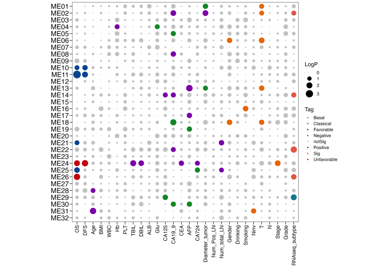
3.5 (e) Kaplan-Meier curves
Kaplan-Meier curves comparing OS between patient subgroups stratified by both adjuvant therapy and the high/low abundance (median cutoff) of ME11. P-values were calculated using the log-rank test, and the hazard ratios calculated using the univariable Cox regression analysis.
library(survival)
library(survminer)
#----------------------------------------------------------------------------------
#  Step 1: Load the data
#----------------------------------------------------------------------------------
# (1) Sample information and clinical characteristics of the 191 PDAC patients (the RJ-cohort 1)
rj1.cohort <- read.xlsx("./data/Extended Data Table 2.xlsx", startRow = 2)
#           ID     Proteomic_ID        RNAseq_ID Age Gender      BMI
# 1 RJ-01-0020 RJ-01-0020-T_PRO RJ-01-0020-T_RNA  61 Female 19.63000
# 2 RJ-01-0038 RJ-01-0038-T_PRO RJ-01-0038-T_RNA  73   Male 22.46003
# 3 RJ-01-0050 RJ-01-0050-T_PRO RJ-01-0050-T_RNA  69 Female 17.63085
# 4 RJ-01-0069 RJ-01-0069-T_PRO RJ-01-0069-T_RNA  69 Female 17.48179

# (2) Scores of the 32 modules in TACs and PDACs of RJ-cohort 1.
module.ssgsea.pro.all <- read.xlsx("./data/Extended Data Table 4.xlsx", sheet = 2, startRow = 2, rowNames = T)
module.ssgsea.pro.all <- t(module.ssgsea.pro.all)
#      RJ-01-0143-N_PRO RJ-01-0768-N_PRO RJ-01-0697-N_PRO RJ-01-0609-N_PRO RJ-01-1055-N_PRO
# ME01       0.34742611      0.253253916       0.28390477       0.32067554      0.325797851
# ME02      -0.11467744      0.009051615      -0.03296699      -0.08755935     -0.096947986
# ME03      -0.04291552     -0.035855079      -0.02943711      -0.05749618      0.016639009
# ME04       0.06708347      0.034863920       0.05803330       0.10310726      0.007498371
# ME05       0.19099018      0.100153070       0.14246697       0.16675071      0.127932887
# ME06       0.03893163      0.240865770       0.14178269       0.07618613      0.038306853
#----------------------------------------------------------------------------------
#  Step 2: Overall survival stratified by ME11
#----------------------------------------------------------------------------------
plot.cohort <- rj1.cohort
plot.cohort <- plot.cohort %>%
                    mutate(ME11_pro = as.numeric(module.ssgsea.pro.all["ME11", Proteomic_ID]),
                           ME11_pro_l = ifelse(ME11_pro>=median(ME11_pro),"High","Low"),
                           ME11_pro_l = factor(as.character(ME11_pro_l), levels = c("Low","High"))) %>%
                    mutate(Censoring_chemo_rev = Censoring_chemo,
                           Censoring_chemo = factor(as.character(Censoring_chemo), levels = c("Chem","NoChem")),
                           Censoring_chemo_rev = factor(as.character(Censoring_chemo_rev), levels = c("NoChem","Chem")))
# coxph
info <- summary(coxph(Surv(OS_month, OS_status) ~ ME11_pro_l, data = plot.cohort))
anno.text <- ""
for (i in 1:nrow(info$conf.int)) {
  anno.text <- paste0(anno.text, "\n", paste0(rownames(info$conf.int)[i], " HR=", round(info$conf.int[i, 1], 3), " CI=", round(info$conf.int[i, 3], 3), "-", round(info$conf.int[i, 4], 3), " P=", signif(info$coefficients[i, 5], 4) ))
}
anno.text <- paste0(anno.text, "\nKaplan-Meier P=", signif(survdiff(Surv(OS_month, OS_status) ~ ME11_pro_l, data = plot.cohort)$pvalue, 4) )
anno.text <- str_replace_all(anno.text, "ME11_pro_l", "")
fit <- survfit(Surv(OS_month, OS_status) ~ ME11_pro_l, data = plot.cohort)
p1 <- ggsurvplot(fit,
                 data = plot.cohort,
                 xlab = 'Time (Months)',
                 pval = TRUE,
                 risk.table = TRUE,
                 risk.table.height = 0.28,
                 conf.int.alpha = 0.05,
                 conf.int = TRUE,
                 palette = c("#00599F","#d80700"),
                 axes.offset = TRUE,
                 break.time.by = 12,  xlim = c(0, 48),
                 title= paste0("OS ME11_pro_l \n", anno.text))
#----------------------------------------------------------------------------------
#  Step 2: KM curve in adjuvant therapy patients stratified by ME11
#----------------------------------------------------------------------------------
plot.cohort.sub <- plot.cohort %>% filter(Censoring_chemo == "Chem") %>%
                          mutate(ME11_pro_l = ifelse(ME11_pro>= median(ME11_pro),"High","Low"),
                                 ME11_pro_l = factor(as.character(ME11_pro_l), levels = c("Low","High")))
info <- summary(coxph(Surv(OS_month, OS_status) ~ ME11_pro_l, data = plot.cohort.sub))
anno.text <- ""
for (i in 1:nrow(info$conf.int)) {
  anno.text <- paste0(anno.text, "\n", paste0(rownames(info$conf.int)[i], " HR=", round(info$conf.int[i, 1], 3), " CI=", round(info$conf.int[i, 3], 3), "-", round(info$conf.int[i, 4], 3), " P=", signif(info$coefficients[i, 5], 4) ))
}
anno.text <- paste0(anno.text, "\nKaplan-Meier P=", signif(survdiff(Surv(OS_month, OS_status) ~ ME11_pro_l, data = plot.cohort.sub)$pvalue, 4) )
anno.text <- str_replace_all(anno.text, "ME11_pro_l", "")
fit <- survfit(Surv(OS_month, OS_status) ~ ME11_pro_l, data = plot.cohort.sub)
p2 <- ggsurvplot(fit,
                 data = plot.cohort.sub,
                 xlab = 'Time (Months)',
                 pval = TRUE,
                 risk.table = TRUE,
                 risk.table.height = 0.28,
                 conf.int.alpha = 0.05,
                 conf.int = TRUE,
                 palette = c("#00599F","#d80700"),
                 axes.offset = TRUE,
                 break.time.by = 12,  xlim = c(0, 48),
                 title= paste0("OS ME11_pro_l Chem \n", anno.text))
#----------------------------------------------------------------------------------
#  Step 2: KM curve in no adjuvant therapy patients stratified by ME11
#----------------------------------------------------------------------------------
plot.cohort.sub <- plot.cohort %>% filter(Censoring_chemo == "NoChem") %>%
                      mutate(ME11_pro_l = ifelse(ME11_pro >= median(ME11_pro),"High","Low"),
                             ME11_pro_l = factor(as.character(ME11_pro_l), levels = c("Low","High")))
info <- summary(coxph(Surv(OS_month, OS_status) ~ ME11_pro_l, data = plot.cohort.sub))
anno.text <- ""
for (i in 1:nrow(info$conf.int)) {
  anno.text <- paste0(anno.text, "\n", paste0(rownames(info$conf.int)[i], " HR=", round(info$conf.int[i, 1], 3), " CI=", round(info$conf.int[i, 3], 3), "-", round(info$conf.int[i, 4], 3), " P=", signif(info$coefficients[i, 5], 4) ))
}
anno.text <- paste0(anno.text, "\nKaplan-Meier P=", signif(survdiff(Surv(OS_month, OS_status) ~ ME11_pro_l, data = plot.cohort.sub)$pvalue, 4) )
anno.text <- str_replace_all(anno.text, "ME11_pro_l", "")
fit <- survfit(Surv(OS_month, OS_status) ~ ME11_pro_l, data = plot.cohort.sub)
p3 <- ggsurvplot(fit,
                 data = plot.cohort.sub,
                 xlab = 'Time (Months)',
                 pval = TRUE,
                 risk.table = TRUE,
                 risk.table.height = 0.28,
                 conf.int.alpha = 0.05,
                 conf.int = TRUE,
                 palette = c("#00599F","#d80700"),
                 axes.offset = TRUE,
                 break.time.by = 12,  xlim = c(0, 48),
                 title= paste0("OS ME11_pro_l NoChem \n", anno.text))
## output
p <- arrange_ggsurvplots(list(p1, p2, p3), ncol = 3, nrow = 1, print = FALSE)
ggsave(paste0("./results/Figure2/Figure2e.pdf"), p, width = 18, height = 8)