4 Figure 3
Fig. 3: Establishing an optimal proteomics-level prognostic risk model using the LASSO-Cox regression. (a) LASSO model for PDAC. The left panel shows the regression coefficients of 14 proteins in the LASSO-Cox regression model. The right heatmap displays the protein abundance of these 14 proteins in each PDAC patient. The bottom scatter plot presents the LASSO score across PDAC patients, with patients ordered according to their LASSO score and stratified into two groups based on the median value of the score. (b) Kaplan-Meier survival curves comparing OS (left) and DFS (right) between LASSO score-low and -high groups in “RJ-cohort 1”. P-value was calculated using the log-rank test. (c) Overlay of the 14 proteins in the LASSO model onto the weighted correlation network nodes. Nodes are colored by functional protein modules (the same as Fig. 2a), and black nodes represent proteins in the LASSO model. (d) Spearman’s correlation between the LASSO score and the enrichment score of the 32 functional modules in “RJ-cohort 1” and Cao et al. cohort. P-values were calculated using spearman’s correlation and adjusted using the BH method. Asterisks (*) indicate adjusted P-value < 0.05. Comprehensive information (including correlation coefficients, P-values, and adjusted P-values) is provided in Extended Data Table 3, e. (e) Kaplan-Meier survival curves comparing OS between LASSO score-low and -high groups using the data from Cao et al cohort. Patients are stratified into two groups based on the median value of the LASSO score. P-value was calculated using the log-rank test. (f) Kaplan-Meier survival curves comparing OS (left) and DFS (right) between LASSO score-low and -high groups in another in-house PDAC cohort (“RJ-cohort 2”). Patients are stratified into two groups based on the median value of the LASSO score. The abundance of 14 proteins was determined by PRM. P-value was calculated using the log-rank test.
4.1 (a) LASSO model for PDAC
We established a prognostic risk model8 for PDAC through the least absolute shrinkage and selection operator (LASSO)-Cox regression analysis. The resulting model contained 14 proteins that stratified PDAC patients into two groups based on their LASSO scores, namely, score-high and score-low.
library(glmnet)
library(openxlsx)
library(survminer)
library(survival)
library(tidyverse)
library(RColorBrewer)
library(ComplexHeatmap)
library(forestmodel)
library(ROCR)
dir.create("./results/Figure3/lasso",recursive = T)
#----------------------------------------------------------------------------------
#  Step 1: load data
#----------------------------------------------------------------------------------
## PDAC Tumor proteomics
pdac.pro  <- readRDS('./data/proteomics/20230412_PDAC_PRO_exp.rds')
pdac.pro  <- pdac.pro [,grep('_T_',colnames(pdac.pro))]   %>% t() %>% as.data.frame() # 191 tumor samples * 4787 protein
## WGCNA protein
wgcna <- readRDS("./data/proteomics/wgcna/2D-node.data.rds")
pdac.pro <- pdac.pro [,intersect(wgcna$Gene,colnames(pdac.pro))] #  191 samples * 3906 protein
## PDAC clinical data
cli.pdac <- readRDS('./data/clinical/20230412_PDAC_191_patients_clinical.rds')
rownames(cli.pdac) <- cli.pdac$ID
## Lasso data
y.train <- data.frame(time=cli.pdac$Time_OS,
                      status=cli.pdac$Censoring_OS,
                      row.names = row.names(cli.pdac)) %>%
           na.omit(y.train) %>%
           as.matrix()
x.train <- pdac.pro[row.names(y.train),] %>% as.matrix() %>% na.omit()
y.train <- y.train[row.names(x.train),]
#----------------------------------------------------------------------------------
#  Step 2: Fit the Lasso Regression Model
#----------------------------------------------------------------------------------
set.seed(1000)
fit <-glmnet(x=x.train,
             y=y.train,
             family = "cox",  # cox : cox , binomial : logistic
             alpha  = 1)      # 1 : lasso penalty, 0 : ridge penalty.
pdf('./results/Figure3/lasso/0.Coefficients.pdf',width = 5,height = 4)
plot(fit,xvar="lambda",label=F)
dev.off()
# Cross-validation
cvfit <- cv.glmnet(x=x.train,
                   y=y.train,
                   family = "cox",
                   type.measure="deviance",
                   alpha  = 1,
                   nfolds = 10)
png(paste0('./results/Figure3/lasso/S5A-Coeff.png'), width = 5,height = 5,res=1200,units="in")
plot(fit,xvar="lambda",label=F)
abline(v = log(cvfit$lambda.min), col = "black",lty=2)
text(-4,-4, labels = paste0("lambda.min:  ", round(cvfit$lambda.min,4)),col = "black",cex = 0.75)
dev.off()
png(paste0('./results/Figure3/lasso/S5B-cvfit.png'), width = 5,height = 5,res=1200,units="in")
plot(cvfit)
text(-3,250, labels = paste0("lambda.min:  ", round(cvfit$lambda.min,4)),col = "red",cex = 0.75)
text(-3,200, labels = paste0("lambda.1se:  ", round(cvfit$lambda.1se,4)),col = "black",cex = 0.75)
dev.off()
#----------------------------------------------------------------------------------
#  Step 3: Best Lasso model
#----------------------------------------------------------------------------------
lasso_best <- glmnet(x = x.train,
                     y = y.train,
                     alpha = 1,
                     lambda = cvfit$lambda.min,
                     nfolds = 10,
                     family = "cox")
gene.coef  <- as.matrix(round(coef(lasso_best), 4))
coef.lasso <- gene.coef[which(gene.coef[, 1] != 0), ]
coef.lasso <- data.frame(genes=names(coef.lasso),
                   coefficient=as.numeric(coef.lasso)) %>% arrange(-coefficient)
write.xlsx(coef.lasso, "./results/Figure3/lasso/2.coef_PDAC.Pro.xlsx", rowNames = F,colNames = T,overwrite = T)
## Lasso score
y <- as.data.frame(y.train) %>%
mutate(LassoScore=predict(lasso_best,s=cvfit$lambda.min,newx=x.train)) %>%
mutate(LassoScore=as.numeric(LassoScore), ID=rownames(y.train))
y <- y %>% mutate(LASSO.level=ifelse(LassoScore>median(LassoScore),"High" ,"Low")) %>%
mutate(LASSO.level=factor(LASSO.level,levels = c( "Low","High"))) ## cutoff : median
write.xlsx(y,paste0('./results/Figure3/lasso/3.Lasso_Score.xlsx'),rowNames = T,colNames = T,overwrite = T)
#----------------------------------------------------------------------------------
# Step 4: Visualization
#----------------------------------------------------------------------------------
## bar plot : gene cofficient
df.coef <- coef.lasso
rownames(df.coef) <- df.coef$genes
df.coef <- df.coef %>% transmute(gene=genes,cor=coefficient) %>%
mutate(gene=paste0(gene," (",cor,")")) %>%
arrange(cor) %>%
mutate(gene=factor(gene,levels = gene)) %>%
mutate(group=ifelse(cor>0,"A","B"))
p1 <- ggplot(df.coef, aes(gene, cor, fill = group)) +
geom_bar(stat = 'identity') +
ylab('coefficient') +
xlab('') +
guides(colour=F,fill=F) +
theme_bw(base_size = 12) +
scale_fill_manual(values = brewer.pal(9,'Set1')) +
theme(panel.grid =element_blank(),
axis.text = element_text(colour = 'black'),
axis.text.x = element_text(size = 8)) +
coord_flip()
ggsave("./results/Figure3/5A-Lasso_cofficient_barplot.png",p1,width = 3,height = 4)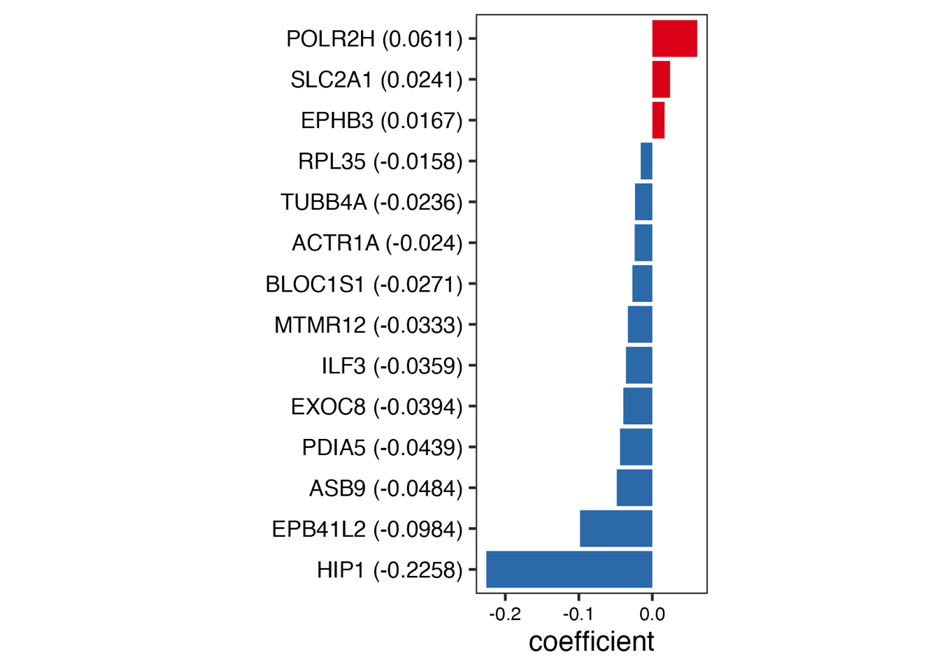
## dot plot : lasso score
df.score <- y
df.score <- df.score %>% mutate(samples=rownames(df.score))  %>%
                arrange(LassoScore) %>%
                mutate(samples=factor(samples,levels = samples))
p2 <- ggscatter(df.score, x="samples", y="LassoScore", color = "LASSO.level",
                palette = c("#0ac9c9","#ea358d"))+
  geom_hline(yintercept=median(df.score$LassoScore), linetype=2,color='black') +
  geom_vline(xintercept=median(1:nrow(df.score))+0.5, linetype=2,color='black') +
  annotate('text',
           x=median(1:nrow(df.score))+15,
           y=median(df.score$LassoScore)+0.5,
           label=paste0('cutoff: ', round(median(df.score$LassoScore),4)),size=5, color='black') +
  ylab('PDAC Score') +
  xlab('')
ggsave("./results/Figure3/5A-Lasso_score_dotplot.png",p2,width = 8,height = 4)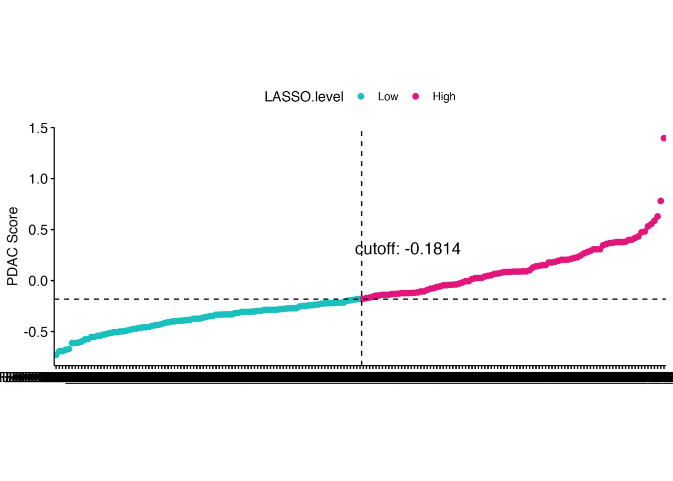
## Heatmap : protein abundance
heat.data <- t(x.train)
heat.data <- heat.data[rev(rownames(df.coef)),row.names(df.score)]
heat.data <- t(scale(t(heat.data)))
png("./results/Figure3/5A-Lasso_gene_heatmap.png",width = 8,height = 4,res=1200,units="in")
p3 <- Heatmap(heat.data, name = "Z-score",
              col = colorRampPalette(c("#00599F","#1c7ec9","#FFFFFF",
                                        "#e53f39","#D01910"))(100),
              cluster_rows = F,cluster_columns = F,show_column_names = F)
draw(p3)
dev.off()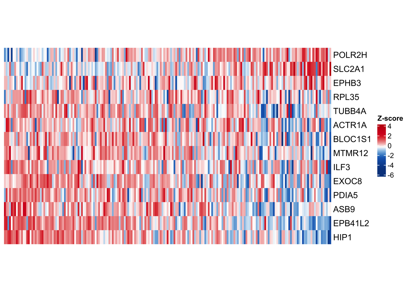
#----------------------------------------------------------------------------------
#  Step 5: receiver operating characteristic (ROC)
#----------------------------------------------------------------------------------
# performance of model
lasso.prob <- predict(cvfit, newx=x.train , family = "cox",
                      s=c(cvfit$lambda.min, cvfit$lambda.1se) )
re <- cbind(as.data.frame(y.train),lasso.prob)  %>% as.data.frame()
colnames(re) <- c('time','status','prob_min','prob_1se')
# model: lambda.min
pred_min <- prediction(predictions=re$prob_min, labels=re$status) # predictions: containing the prediction. labels: true class labels
perf_min <- performance(pred_min,"tpr","fpr")
auc_min  <- performance(pred_min,"auc")@y.values[[1]]
# mocel: lambda.1se
pred_1se <- prediction(re$prob_1se, re$status)
perf_1se <- performance(pred_1se,"tpr","fpr")
auc_1se  <- performance(pred_1se,"auc")@y.values[[1]]
## plot
png(paste0('./results/Figure3/lasso/S5C-ROC.png'), width = 5,height = 5,res=1200,units="in")
plot(perf_min,colorize=F, col="red")
plot(perf_1se,colorize=F, col="blue",add = T)
lines(c(0,1),c(0,1), col = "gray", lty = 4 )
text(0.7,0.3, labels = paste0("lambda.min: AUC=", round(auc_min,2)),col = "red")
dev.off()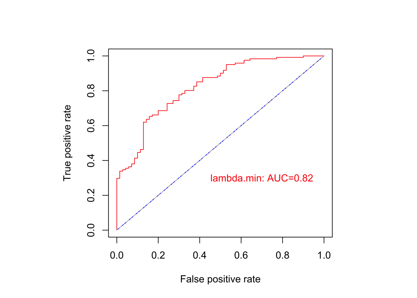
#----------------------------------------------------------------------------------
#  Step 6: Multivariate analysis
#----------------------------------------------------------------------------------
# data
y_forest <- y %>% left_join(cli.pdac , by =c('ID'='ID'))
y_forest <- y_forest %>% select(  c('time','status','LASSO.level',
                        'age','gender','CA125',
                        'CA19_9','CEA','Smoking',"Drinking",'AJCC_V8',
                        'Censoring_chemo'))
y_forest <- y_forest %>% rename(LassoLevel=LASSO.level,
                                Age=age,Gender=gender,
                                CA199=CA19_9,
                                Adjuvant_therapy=Censoring_chemo,
                                AJCC_stage=AJCC_V8)
y_forest <- y_forest %>% mutate(Gender=factor(Gender,levels = c("Female","Male")))
# AJCC_stage
table(y_forest$AJCC_stage)
a <- y_forest$AJCC_stage
b <- recode(a, Ia = "I", Ib = "I",IIa= "II", IIb= "II",III="III",IV="IV")
y_forest$AJCC_stage <- factor(b,levels = c("I","II","III"))
# coxph
cfit <- coxph(Surv(time,status)~LassoLevel+Age+Gender+CA125+CA199+
                CEA+Smoking+Drinking+AJCC_stage+Adjuvant_therapy,
              data = y_forest)
# Forest plots
p <- forest_model(cfit,
      format_options = forest_model_format_options(colour = brewer.pal(9,'Set1')[2],                 shape = 16,text_size =  15,point_size = 2.5, banded = T),
      factor_separate_line = F )
ggsave(paste0("./results/Figure3/S5D-multivariate_forest.png"), p,  width = 8, height = 6)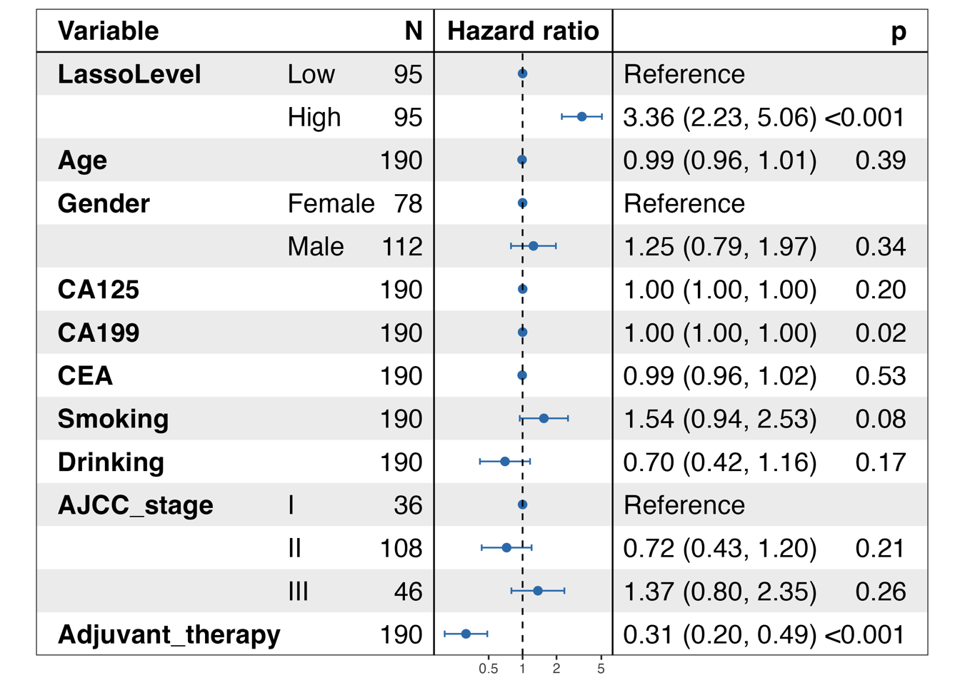
4.2 (b) Kaplan-Meier curves in OS/DFS
Kaplan-Meier curves comparing OS (left) and DFS (right) between LASSO score-low and -high groups in “RJ cohort-1”. P-value was calculated using the log-rank test.
#----------------------------------------------------------------------------------
#  Step 1: Loading data
#----------------------------------------------------------------------------------
# (1) Sample information and clinical characteristics of the 191 PDAC patients (the RJ-cohort 1)
rj1.cohort <- read.xlsx("./data/Extended Data Table 2.xlsx", startRow = 2)
#           ID     Proteomic_ID        RNAseq_ID Age Gender      BMI DM Smoking
# 1 RJ-01-0020 RJ-01-0020-T_PRO RJ-01-0020-T_RNA  61 Female 19.63000  1       0
# 2 RJ-01-0038 RJ-01-0038-T_PRO RJ-01-0038-T_RNA  73   Male 22.46003  0       0
# 3 RJ-01-0050 RJ-01-0050-T_PRO RJ-01-0050-T_RNA  69 Female 17.63085  0       0
# 4 RJ-01-0069 RJ-01-0069-T_PRO RJ-01-0069-T_RNA  69 Female 17.48179  1       0
# 5 RJ-01-0070 RJ-01-0070-T_PRO RJ-01-0070-T_RNA  65   Male 23.43750  0       0
# 6 RJ-01-0074 RJ-01-0074-T_PRO RJ-01-0074-T_RNA  61   Male 23.66144  0       0
rj1.cohort <- rj1.cohort %>%  mutate(LassoLevel=factor(as.character(LassoLevel), levels = c("Low","High")))
color.bin.lasso <- c("#00599F","#d80700")
#----------------------------------------------------------------------------------
#  Step 2: OS survival stratified by lasso level
#----------------------------------------------------------------------------------
info <- summary(coxph(Surv(OS_month, OS_status) ~ LassoLevel, data = rj1.cohort))
anno.text <- ""
for (i in 1:nrow(info$conf.int)) {
  anno.text <- paste0(anno.text, "\n", paste0(rownames(info$conf.int)[i], " HR=", round(info$conf.int[i, 1], 3), " CI=", round(info$conf.int[i, 3], 3), "-", round(info$conf.int[i, 4], 3), " P=", signif(info$coefficients[i, 5], 4) ))
}
anno.text <- paste0(anno.text, "\nKaplan-Meier P=", signif(survdiff(Surv(OS_month, OS_status) ~ LassoLevel, data = rj1.cohort)$pvalue, 4) )
anno.text <- str_replace_all(anno.text, "LassoLevel", "")
fit <- survfit(Surv(OS_month, OS_status) ~ LassoLevel, data = rj1.cohort)
p1 <- ggsurvplot(fit,
                 data = rj1.cohort,
                 xlab = 'Time (Months)',
                 pval = TRUE,
                 risk.table = TRUE,
                 risk.table.height = 0.28,
                 conf.int.alpha = 0.05,
                 conf.int = TRUE,
                 palette = color.bin.lasso,
                 axes.offset = TRUE,
                 break.time.by = 12,  xlim = c(0, 48),
                 title= paste0("OS LassoLevel \n", anno.text))
#----------------------------------------------------------------------------------
#  Step 2: DFS survival stratified by lasso level
#----------------------------------------------------------------------------------
info <- summary(coxph(Surv(DFS_month, DFS_status) ~ LassoLevel, data = rj1.cohort))
anno.text <- ""
for (i in 1:nrow(info$conf.int)) {
  anno.text <- paste0(anno.text, "\n", paste0(rownames(info$conf.int)[i], " HR=", round(info$conf.int[i, 1], 3), " CI=", round(info$conf.int[i, 3], 3), "-", round(info$conf.int[i, 4], 3), " P=", signif(info$coefficients[i, 5], 4) ))
}
anno.text <- paste0(anno.text, "\nKaplan-Meier P=", signif(survdiff(Surv(DFS_month, DFS_status) ~ LassoLevel, data = rj1.cohort)$pvalue, 4) )
anno.text <- str_replace_all(anno.text, "LassoLevel", "")
fit <- survfit(Surv(DFS_month, DFS_status) ~ LassoLevel, data = rj1.cohort)
p2 <- ggsurvplot(fit,
                 data = rj1.cohort,
                 xlab = 'Time (Months)',
                 pval = TRUE,
                 risk.table = TRUE,
                 risk.table.height = 0.28,
                 conf.int.alpha = 0.05,
                 conf.int = TRUE,
                 palette = color.bin.lasso,
                 axes.offset = TRUE,
                 break.time.by = 12,  xlim = c(0, 48),
                 title= paste0("DFS LassoLevel \n", anno.text))
## output
p <- arrange_ggsurvplots(list(p1, p2), ncol = 2, nrow = 1, print = FALSE)
ggsave(paste0("./results/Figure3/Figure3b.pdf"), p, width = 16, height = 10)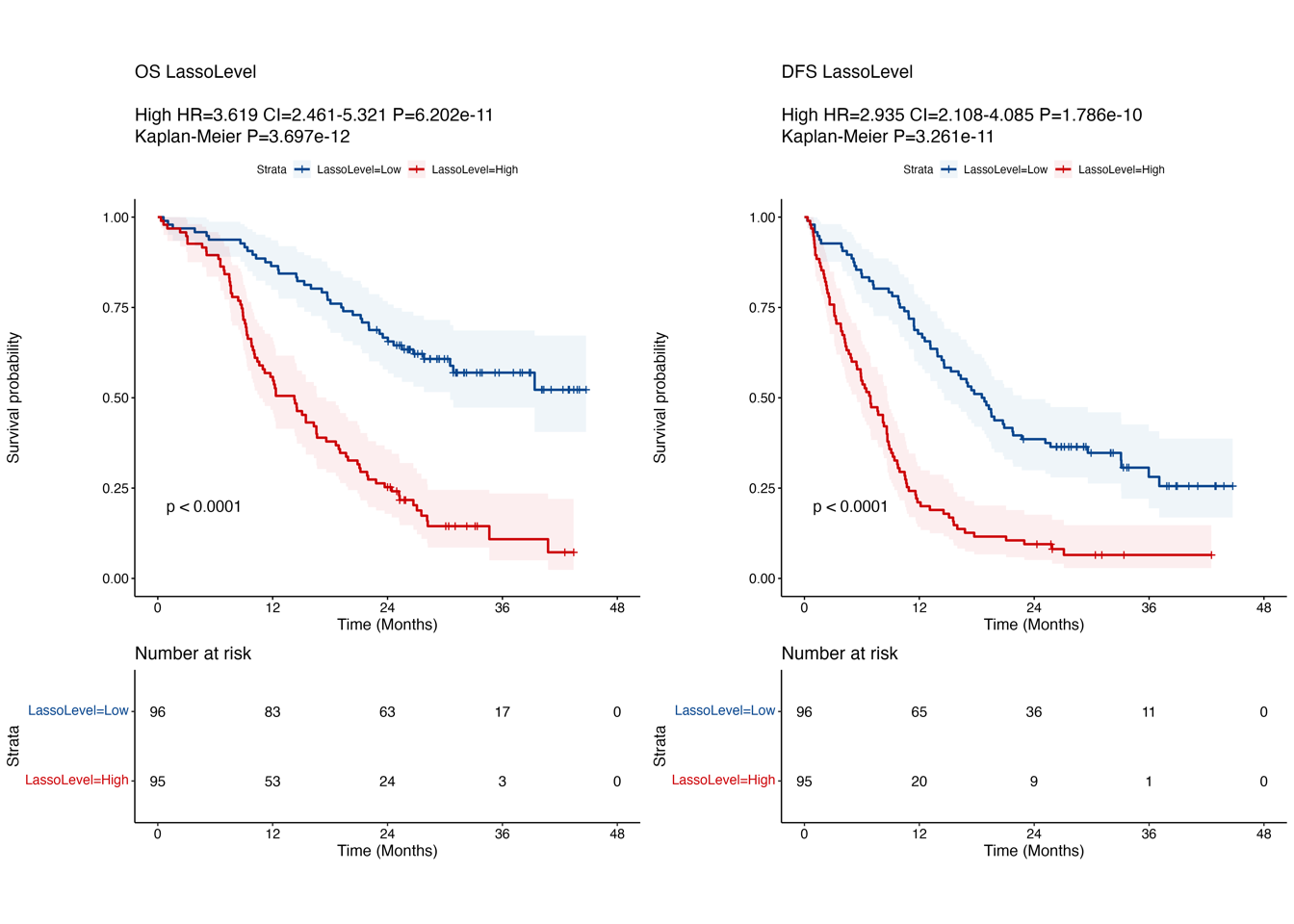
4.3 (c) Lasso proteins in module
Overlay of the 14 proteins in the LASSO model onto the weighted correlation network nodes. Nodes are colored by functional protein modules (the same as Fig. 2a), and black nodes represent proteins in the LASSO model.
## data
node.data <- readRDS("./data/proteomics/wgcna/2D-node.data.rds")
edge.data <- readRDS("./data/proteomics/wgcna/2D-edge.data.rds")
## lasso gene plot
color.module <- c("#ecb888","#af88bb","#a032cb","#efbed6","#fc496a","#b6d37f","#589336","#7fd68e","#52c465","#3372e0","#84d7f6","#5394c3","#6376b3","#7f6cd7","#c4ceff","#fc9d40","#5c95e0","#cd7560","#ff70e4", "#ff8738", "#ffcead","#1cbf8b", "#b76d38", "#1584ff", "#7f006d", "#ffd35f","#E66F73","#F57F20","#1DBB95","#9CB79F","#F0B8D2","#A0485E","#A0688E","#C7E1DF","#51B1DF","#6D97D7","#5D6193","#CEC3E0","#A9917E","#7C7D80","#F4E192","#ADD666")
gg <- ggplot()
gg <- gg + geom_segment(mapping = aes(x = from.x, y = from.y, xend = to.x, yend = to.y), color = "#CCCCCC", size = 0.01, data = edge.data)
gg <- gg + geom_point(mapping = aes(x = pos.x, y = pos.y, color = Module), size = 1, data = node.data)
gg <- gg + geom_point(mapping = aes(x = pos.x, y = pos.y, color = Module), fill = "red", size = 5, shape = 21, data = node.data[which(node.data$ISlassoGene == "yes"), ])
gg <- gg + geom_text(mapping = aes(x = pos.x, y = pos.y, label = Gene), size = 5, color = "black", data = node.data[which(node.data$ISlassoGene == "yes"), ])
gg <- gg + scale_size(range = c(0, 6) * 2)
gg <- gg + theme_void()
gg <- gg + labs(x = "", y = "", title = paste0("color by ISlassoGene"))
gg <- gg + scale_colour_manual(values = color.module)
gg <- gg + theme(legend.position = "none")
ggsave(paste0("./results/Figure3/3c-Lasso_gene_in_module.png"), gg, width = 8, height = 8.2)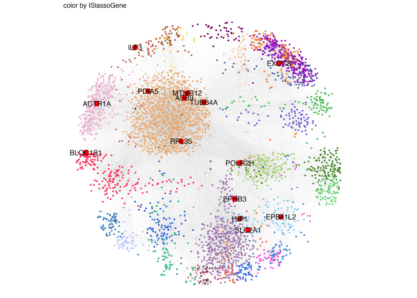
4.4 (d) LassoScore~ModuleScore
Spearman’s correlation between the LASSO score and the enrichment score of the 32 functional modules in “RJ-cohort 1” and Cao et al cohort. P-values were calculated using spearman’s correlation and adjusted using BH method.
library(ggcorrplot)
#----------------------------------------------------------------------------------
#  Step 1: Load the Data
#----------------------------------------------------------------------------------
# (1) Sample information and clinical characteristics of the 191 PDAC patients (the RJ-cohort 1)
rj1.cohort <- read.xlsx("./data/Extended Data Table 2.xlsx", startRow = 2)
#           ID     Proteomic_ID        RNAseq_ID Age Gender      BMI DM Smoking
# 1 RJ-01-0020 RJ-01-0020-T_PRO RJ-01-0020-T_RNA  61 Female 19.63000  1       0
# 2 RJ-01-0038 RJ-01-0038-T_PRO RJ-01-0038-T_RNA  73   Male 22.46003  0       0
# 3 RJ-01-0050 RJ-01-0050-T_PRO RJ-01-0050-T_RNA  69 Female 17.63085  0       0
# 4 RJ-01-0069 RJ-01-0069-T_PRO RJ-01-0069-T_RNA  69 Female 17.48179  1       0
# 5 RJ-01-0070 RJ-01-0070-T_PRO RJ-01-0070-T_RNA  65   Male 23.43750  0       0
# 6 RJ-01-0074 RJ-01-0074-T_PRO RJ-01-0074-T_RNA  61   Male 23.66144  0       0

# (2) Scores of the 32 modules in TACs and PDACs of RJ-cohort 1.
module.ssgsea.pro.all <- read.xlsx("./data/Extended Data Table 4.xlsx", sheet = 2, startRow = 2, rowNames = T)
module.ssgsea.pro.all <- t(module.ssgsea.pro.all)
#      RJ-01-0143-N_PRO RJ-01-0768-N_PRO RJ-01-0697-N_PRO RJ-01-0609-N_PRO RJ-01-1055-N_PRO
# ME01       0.34742611      0.253253916       0.28390477       0.32067554      0.325797851
# ME02      -0.11467744      0.009051615      -0.03296699      -0.08755935     -0.096947986
# ME03      -0.04291552     -0.035855079      -0.02943711      -0.05749618      0.016639009
# ME04       0.06708347      0.034863920       0.05803330       0.10310726      0.007498371
# ME05       0.19099018      0.100153070       0.14246697       0.16675071      0.127932887
# ME06       0.03893163      0.240865770       0.14178269       0.07618613      0.038306853
#----------------------------------------------------------------------------------
#  Step 2:  Spearman correlation : lasso score ~ module score
#----------------------------------------------------------------------------------
plot.mat <- data.frame(t(module.ssgsea.pro.all[, rj1.cohort$Proteomic_ID]), LassoScore = rj1.cohort[, c("LassoScore")] )
corr <- cor(plot.mat, use = "complete.obs", method = "spearman")
p.mat <- cor_pmat(plot.mat, use = "complete.obs", method = "spearman")
p.adj <- p.mat
for (i in 1:ncol(p.adj)) {
  p.adj[, i] <- p.adjust(p.adj[, i], method = "fdr")
}
write.xlsx(list(Corr = corr, p.mat = p.mat, p.adj = p.adj), "./results/Figure3/Figure3d-1.xlsx", overwrite = T, rowNames = T)
# plot
pdf(paste0("./results/Figure3/Figure3d-1.pdf"), width = 10, height = 10)
corrplot::corrplot(corr[, ], method = "ellipse",
                   col = colorRampPalette(c("#1B3361","#76C7FF","#FFFFFF","#FF987A","#6A0D28"))(200))
dev.off()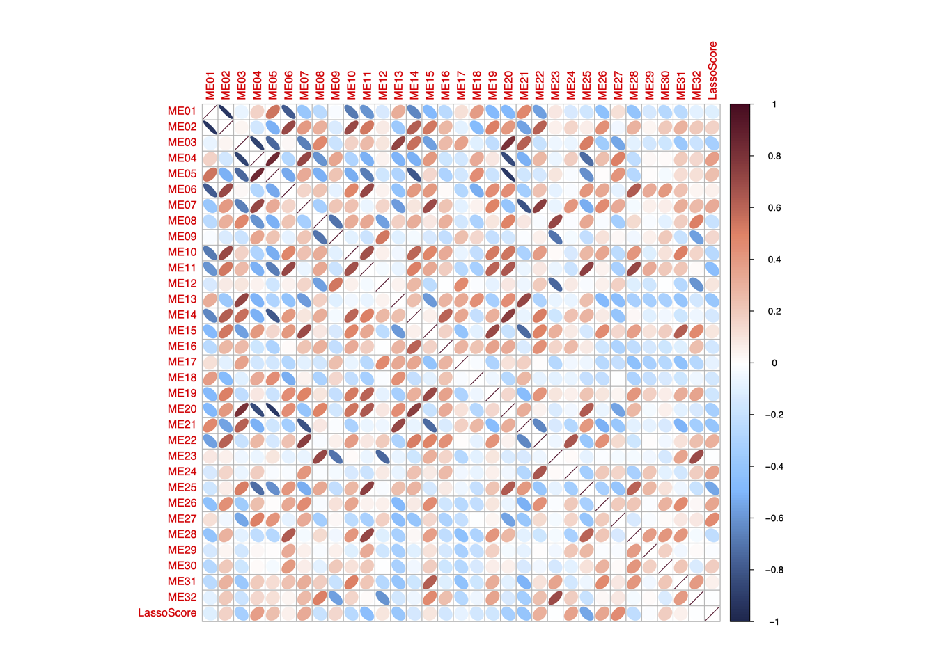
#----------------------------------------------------------------------------------
#  Step 3:  Spearman correlation : lasso score ~ module score in Cao et al cohort
#----------------------------------------------------------------------------------
module.ssgsea.pro.cell <- readRDS("./data/Figure2/cao.module.ssgsea.pro.rds")
cell.meta.data <- read.xlsx("./data/Figure2/cao.meta.data.xlsx")
cell.meta.data$LassoLevel <- factor(as.character(cell.meta.data$LassoLevel), levels = c("Low","High"))
plot.mat <- data.frame(t(module.ssgsea.pro.cell[, cell.meta.data$Proteomic_ID]), LassoScore = cell.meta.data[, c("LassoScore")] )
# Spearman correlation
corr <- cor(plot.mat, use = "complete.obs", method = "spearman")
p.mat <- cor_pmat(plot.mat, use = "complete.obs", method = "spearman")
p.adj <- p.mat
for (i in 1:ncol(p.adj)) {
  p.adj[, i] <- p.adjust(p.adj[, i], method = "fdr")
}
write.xlsx(list(Corr = corr, p.mat = p.mat, p.adj = p.adj), "./results/Figure3/Figure3d-2.xlsx", overwrite = T, rowNames = T)
# plot
pdf(paste0("./results/Figure3/Figure3d-2.pdf"),  width = 10, height = 10)
corrplot::corrplot(corr[, ], method = "ellipse",
                   col = colorRampPalette(c("#1B3361","#76C7FF","#FFFFFF","#FF987A","#6A0D28"))(200))
dev.off()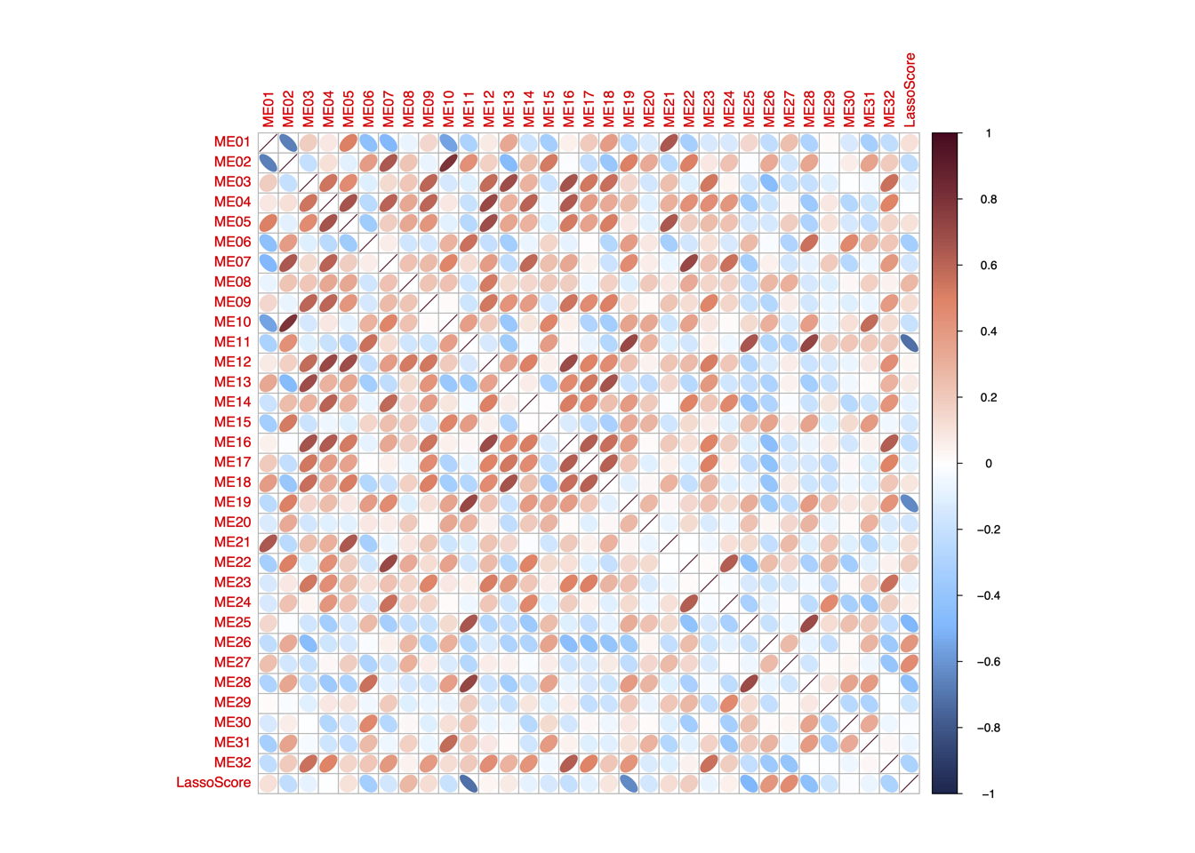
4.5 (e) Cao et al validation
Kaplan-Meier curves comparing OS between LASSO score-low and -high groups using the data from Cao et al cohort. Patients are stratified into two groups based on the median value of the LASSO score. P-value was calculated using the log-rank test.
## data
cell.meta.data <- read.xlsx("./data/Figure2/cao.meta.data.xlsx")
color.bin.lasso <- c("#00599F","#d80700")
cell.meta.data <- cell.meta.data %>% mutate(LassoLevel=factor(LassoLevel,level=c("Low","High")))
## coxph
info <- summary(coxph(Surv(OS_month, OS_status) ~ LassoLevel, data = cell.meta.data))
anno.text <- ""
for (i in 1:nrow(info$conf.int)) {
  anno.text <- paste0(anno.text, "\n", paste0(rownames(info$conf.int)[i], " HR=", round(info$conf.int[i, 1], 3), " CI=", round(info$conf.int[i, 3], 3), "-", round(info$conf.int[i, 4], 3), " P=", signif(info$coefficients[i, 5], 4) ))
}
anno.text <- paste0(anno.text, "\nKaplan-Meier P=", signif(survdiff(Surv(OS_month, OS_status) ~ LassoLevel, data = cell.meta.data)$pvalue, 4) )
anno.text <- str_replace_all(anno.text, "LassoLevel", "")
fit <- survfit(Surv(OS_month, OS_status) ~ LassoLevel, data = cell.meta.data)
p1 <- ggsurvplot(fit,
                 data = cell.meta.data,
                 xlab = 'Time (Months)',
                 pval = TRUE,
                 risk.table = TRUE,
                 risk.table.height = 0.28,
                 conf.int.alpha = 0.05,
                 conf.int = TRUE,
                 palette = color.bin.lasso,
                 axes.offset = TRUE,
                 break.time.by = 12,  xlim = c(0, 48),
                 title= paste0("OS LassoLevel \n", anno.text))
p <- arrange_ggsurvplots(list(p1), ncol = 1, nrow = 1, print = FALSE)
ggsave(paste0("./results/Figure3/Figure3e.pdf"), p, width = 8, height = 10)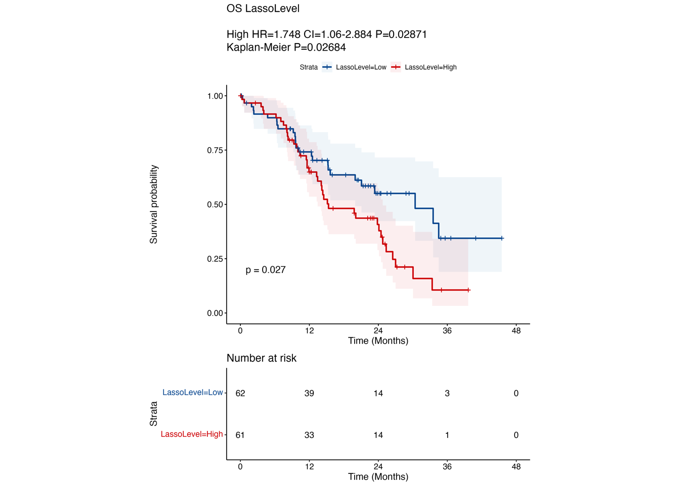
4.6 (f) RJ-cohort 2 validation
Kaplan-Meier curves comparing OS (left) and DFS (right) between LASSO score-low and -high groups in another in-house PDAC cohort (“RJ-cohort 2”). Patients are stratified into two groups based on the median value of the LASSO score. The abundance of 14 proteins was determined by PRM. P-value was calculated using the log-rank test.
#----------------------------------------------------------------------------------
#  Step 1: Load the Data
#----------------------------------------------------------------------------------
# The LASSO score in RJ-cohort 2
rj2.cohort <- read.xlsx("./data/Extended Data Table 5.xlsx", sheet = 3, startRow = 2)
rj2.cohort <- rj2.cohort %>% mutate(LassoLevel=factor(as.character(LassoLevel), levels = c("Low","High")))
color.bin.lasso <- c("#00599F","#d80700")
#----------------------------------------------------------------------------------
#  Step 2: OS survival stratified by lasso level
#----------------------------------------------------------------------------------
info <- summary(coxph(Surv(OS_month, OS_status) ~ LassoLevel, data = rj2.cohort))
anno.text <- ""
for (i in 1:nrow(info$conf.int)) {
  anno.text <- paste0(anno.text, "\n", paste0(rownames(info$conf.int)[i], " HR=", round(info$conf.int[i, 1], 3), " CI=", round(info$conf.int[i, 3], 3), "-", round(info$conf.int[i, 4], 3), " P=", signif(info$coefficients[i, 5], 4) ))
}
anno.text <- paste0(anno.text, "\nKaplan-Meier P=", signif(survdiff(Surv(OS_month, OS_status) ~ LassoLevel, data = rj2.cohort)$pvalue, 4) )
anno.text <- str_replace_all(anno.text, "LassoLevel", "")
fit <- survfit(Surv(OS_month, OS_status) ~ LassoLevel, data = rj2.cohort)
p1 <- ggsurvplot(fit,
                 data = rj2.cohort,
                 xlab = 'Time (Months)',
                 pval = TRUE,
                 risk.table = TRUE,
                 risk.table.height = 0.28,
                 conf.int.alpha = 0.05,
                 conf.int = TRUE,
                 palette = color.bin.lasso,
                 axes.offset = TRUE,
                 break.time.by = 12,  xlim = c(0, 48),
                 title= paste0("OS LassoLevel \n", anno.text))
#----------------------------------------------------------------------------------
#  Step 3: DFS survival stratified by lasso level
#----------------------------------------------------------------------------------
info <- summary(coxph(Surv(DFS_month, DFS_status) ~ LassoLevel, data = rj2.cohort))
anno.text <- ""
for (i in 1:nrow(info$conf.int)) {
  anno.text <- paste0(anno.text, "\n", paste0(rownames(info$conf.int)[i], " HR=", round(info$conf.int[i, 1], 3), " CI=", round(info$conf.int[i, 3], 3), "-", round(info$conf.int[i, 4], 3), " P=", signif(info$coefficients[i, 5], 4) ))
}
anno.text <- paste0(anno.text, "\nKaplan-Meier P=", signif(survdiff(Surv(DFS_month, DFS_status) ~ LassoLevel, data = rj2.cohort)$pvalue, 4) )
anno.text <- str_replace_all(anno.text, "LassoLevel", "")
fit <- survfit(Surv(DFS_month, DFS_status) ~ LassoLevel, data = rj2.cohort)
p2 <- ggsurvplot(fit,
                 data = rj2.cohort,
                 xlab = 'Time (Months)',
                 pval = TRUE,
                 risk.table = TRUE,
                 risk.table.height = 0.28,
                 conf.int.alpha = 0.05,
                 conf.int = TRUE,
                 palette = color.bin.lasso,
                 axes.offset = TRUE,
                 break.time.by = 12,  xlim = c(0, 48),
                 title= paste0("DFS LassoLevelRNA \n", anno.text))
# output
p <- arrange_ggsurvplots(list(p1, p2), ncol = 2, nrow = 1, print = FALSE)
ggsave(paste0("./results/Figure3/Figure3f.pdf"), p, width = 16, height = 10)