OLFML3 BOOKLET
2024-07-18
1 Figure 1
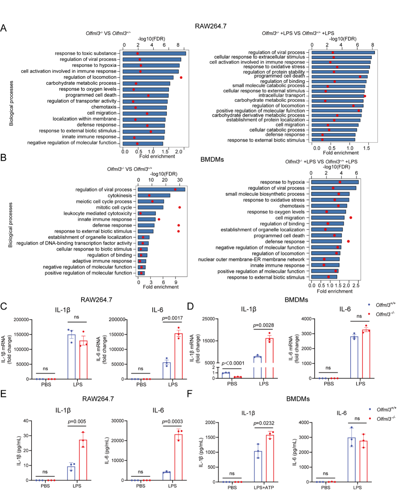
Fig. 1. Evaluation of the effects of Olfml3 knockout on the inflammatory response of macrophages upon LPS stimulation. (A-B) Top biological processes from RNA-Seq analyses of DEGs in RAW264.7 cells (A) and BMDMs (B). The RNA-Seq data are from three biological replicates. The bars and dots dictate fold enrichment and -log values of false discovery rate (FDR) respectively. (C-D) The effects of Olfml3 knockout on IL-1 and IL-6 mRNA expression in RAW264.7 (C) and BMDMs (D), as determined by RT-qPCR. (E-F) The effects of Olfml3 knockout on IL-1 and IL-6 protein levels in culture supernatant of RAW264.7 (E) and BMDMs (F), as determined by ELISA. For C and D, the data are collected at 4 h post LPS stimulation. For E and F, cell supernatant is collected at 24 h after LPS stimulation. Especially, LPS (3 h) and ATP (45 min) induced IL-1 release is measured in BMDMs . The data represent the mean ± SEM of at least three biological replicates and the p values of indicated comparisons are determined using two-tailed Student’s t test. NS, not significant.
1.1 (A) GO analysis in RAW264.7
library(tidyr)
library(ggpubr)
library(ggthemes)
library(patchwork)
library(limma)
library(PIONE)
library(tidyverse)
library(XGR)
dir.create("./results/Figure1/",recursive = T)
#----------------------------------------------------------------------------------
#  Step 1: Load the Data
#----------------------------------------------------------------------------------
# DEGs
ls_limma <- readRDS("./results/FigureS4/FigureS4_A.Limma_fdr0.05_fc1.5.rds")
# Gene ontology
sets <- tibble(onto=c('GOBP','GOCC','GOMF')) %>%
          mutate(set=map(onto,~oRDS(str_c("org.Mm.eg",.x),
          placeholder="http://www.comptransmed.pro/bigdata_ctm")))
# KEGG
kegg <- tibble(onto=c('KEGG')) %>%
          mutate(set=map(onto,~oRDS(str_c("org.Mm.eg",.x),
          placeholder="http://www.comptransmed.pro/bigdata_ctm"))) # 8335 genes
# terms in GO
gobp <- sets$set[1][[1]]$info # 15725 terms , 28555 genes
gocc <- sets$set[2][[1]]$info # 2028 terms
gomf <- sets$set[3][[1]]$info # 4575 terms
# glycolysis
gobp[grep("glycolysis",gobp$name),]
# glucose
gobp[grep("glucose",gobp$name),]
# terms in kegg
kegg.term <- kegg$set[[1]]$info # 350 terms
#----------------------------------------------------------------------------------
#  Step 2: GO analysis
#----------------------------------------------------------------------------------
## (1) KO_WT
# DE genes
deg_vec <- ls_limma[["KO_WT"]] %>% filter(group!="not sig") %>% pull(GeneSymbol) %>% unique()
# enrichment
esad <- oSEAadv(deg_vec, sets, size.range=c(15,1500), test="fisher", min.overlap=3)  ## 最小3
df_eTerm.1 <- esad %>% oSEAextract() %>%
                  #filter(adjp<5e-2, distance==3) %>%
                  mutate(group=namespace) %>% group_by(group) %>%
                  arrange(group,adjp)

## (2) KO.LPS_WT.LPS
# DE genes
deg_vec <- ls_limma[["KO.LPS_WT.LPS"]] %>% filter(group!="not sig") %>% pull(GeneSymbol) %>% unique()
# enrichment
esad <- oSEAadv(deg_vec, sets, size.range=c(15,1500), test="fisher", min.overlap=3)
df_eTerm.2 <- esad %>% oSEAextract() %>%
                  #filter(adjp<5e-2, distance==3) %>%
                  mutate(group=namespace) %>% group_by(group) %>%
                  arrange(group,adjp)
# output
ls_eTerm <- list(KO_WT=df_eTerm.1,
                 KO.LPS_WT.LPS=df_eTerm.2)
ls_eTerm %>% openxlsx::write.xlsx("./results/Figure1/Figure1_A.Enrichment_GO_KO_WT.xlsx")
#----------------------------------------------------------------------------------
#  Step 3: GO analysis visualization
#----------------------------------------------------------------------------------
## (1) KO_WT
df <- read.xlsx("./data/7.RAW-Enrichment_GO_KO_WT.xlsx",sheet = 2)
df <- df %>% arrange(-fc) %>% mutate(name=factor(name,level=rev(name))) %>%
                  mutate(logFDR = -log10(adjp))  %>%
                  mutate(logFDR.plot = logFDR/4 ) # 将要画的第二个轴,先转换到第一个轴的范围内
# plot
p <- ggplot(df, aes(x=name )) +
          geom_col(aes(y=fc),fill = "#3e79b6",color = "black",width = 0.6)  +
          theme_base() +
          coord_flip() +
          geom_point(aes(y=logFDR.plot),fill = "red",color = "red", size = 3)+
          scale_y_continuous(
              # Features of the first axis
              name = "Fold enrichment",
              # Add a second axis and specify its features
              sec.axis = sec_axis(~.*4, name="-log10(FDR)") # 将第二个轴,转换回原数据范围内
              )  +
              ggtitle(label = "Dysregulated GOBP",
                      subtitle = "KO versus WT in RAW") +
              theme(plot.background = element_blank())
ggsave("./results/Figure1/Figure1_A_left.RAW_KO_WT.pdf",p,width = 7,height = 6)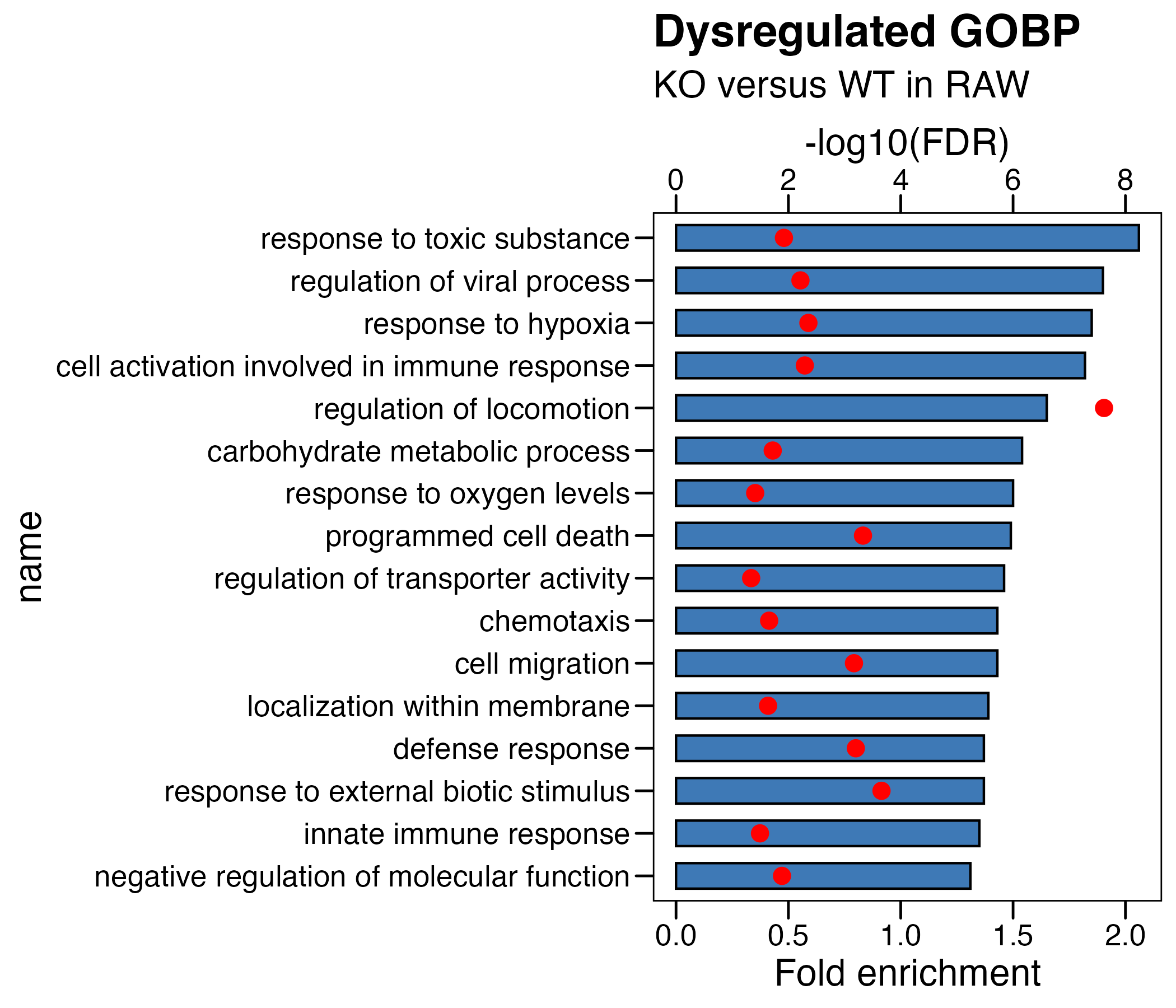
## (2) KO_WT in LPS
df <- read.xlsx("./data/7.RAW-Enrichment_KO.LPS_WT.LPS.xlsx",sheet = 2)
df <- df %>% arrange(-fc) %>% mutate(name=factor(name,level=rev(name))) %>%
                  mutate(logFDR = -log10(adjp))  %>%
                  mutate(logFDR.plot = logFDR/5 ) # 将要画的第二个轴,先转换到第一个轴的范围内
# plot
p <- ggplot(df, aes(x=name )) +
          geom_col(aes(y=fc),fill = "#3e79b6",color = "black",width = 0.6)  +
          theme_base() +
          coord_flip() +
          geom_point(aes(y=logFDR.plot),fill = "red",color = "red", size = 3)+
          scale_y_continuous(
              # Features of the first axis
              name = "Fold enrichment",
              # Add a second axis and specify its features
              sec.axis = sec_axis(~.*5, name="-log10(FDR)") # 将第二个轴,转换回原数据范围内
              )  +
              ggtitle(label = "Dysregulated GOBP",
                      subtitle = "KO.LPS versus WT.LPS in RAW") +
              theme(plot.background = element_blank())
ggsave("./results/Figure1/Figure1_A_right.RAW_KO_WT_LPS.pdf",p,width = 7,height = 6)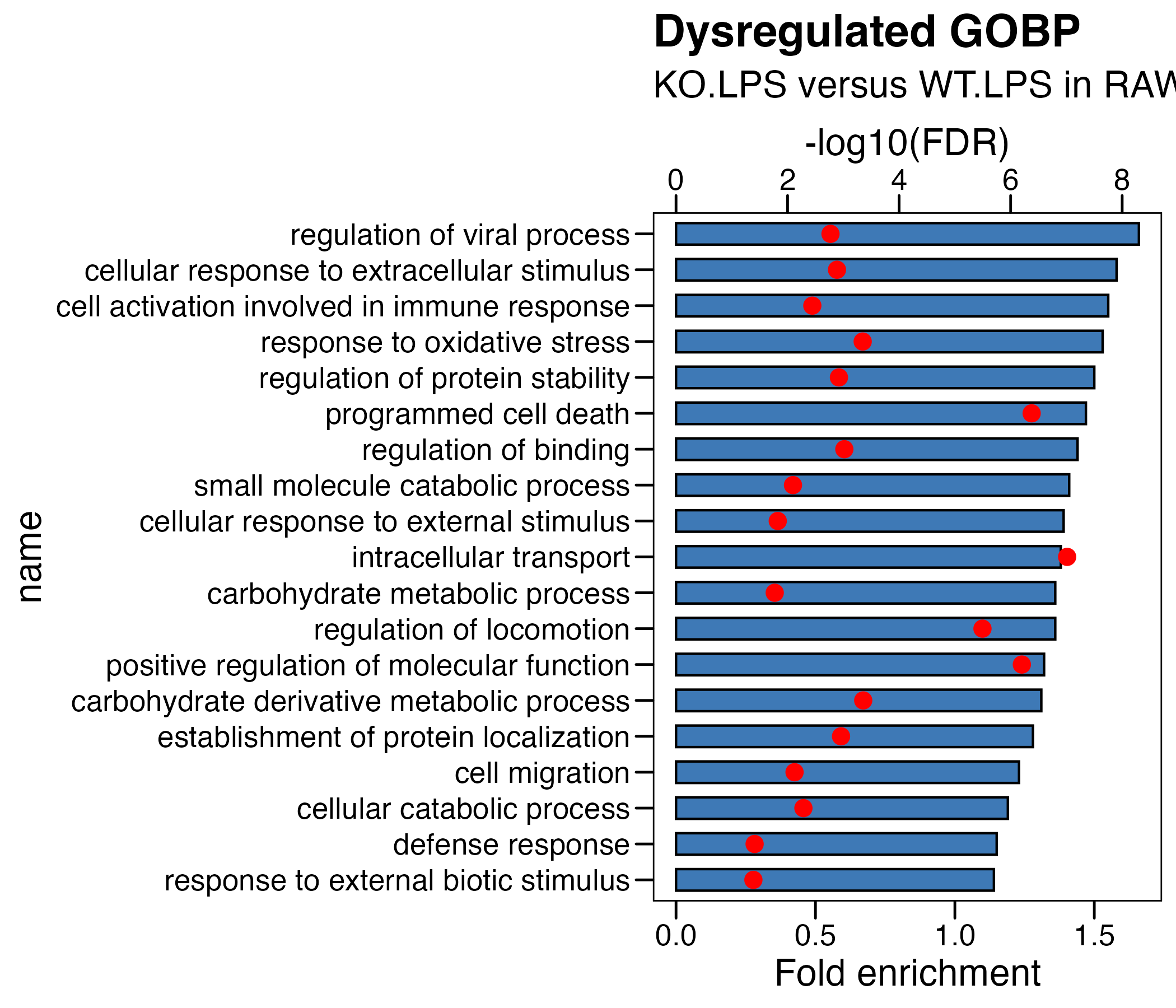
#----------------------------------------------------------------------------------
#  Step 4: KEGG analysis
#----------------------------------------------------------------------------------
## (1) KO_WT
# DE genes
deg_vec <- ls_limma[["KO_WT"]] %>% filter(group!="not sig") %>% pull(GeneSymbol) %>% unique()
# enrichment
esad <- oSEAadv(deg_vec, kegg, size.range=c(15,1500), test="fisher", min.overlap=3)  ## 最小3
df_eTerm.1 <- esad %>% oSEAextract() %>%
                  #filter(adjp<5e-2, distance==3) %>%
                  mutate(group=namespace) %>% group_by(group) %>%
                  arrange(group,adjp)

## (2) KO.LPS_WT.LPS
# DE genes
deg_vec <- ls_limma[["KO.LPS_WT.LPS"]] %>% filter(group!="not sig") %>% pull(GeneSymbol) %>% unique()
# enrichment
esad <- oSEAadv(deg_vec, kegg, size.range=c(15,1500), test="fisher", min.overlap=3)
df_eTerm.2 <- esad %>% oSEAextract() %>%
                  #filter(adjp<5e-2, distance==3) %>%
                  mutate(group=namespace) %>% group_by(group) %>%
                  arrange(group,adjp)


# output
ls_eTerm <- list(KO_WT=df_eTerm.1,
                 KO.LPS_WT.LPS=df_eTerm.2)
ls_eTerm %>% openxlsx::write.xlsx("./results/Figure1/RAW_KEGG_KO_WT.xlsx")
1.2 (B) GO analysis in BMDMs
#----------------------------------------------------------------------------------
#  Step 1: Load the Data
#----------------------------------------------------------------------------------
# DEGs
ls_limma <- readRDS("./results/FigureS4/FigureS4_B.Limma_fdr0.05_fc1.5.rds")
# Gene ontology
sets <- tibble(onto=c('GOBP','GOCC','GOMF')) %>%
          mutate(set=map(onto,~oRDS(str_c("org.Mm.eg",.x),
          placeholder="http://www.comptransmed.pro/bigdata_ctm")))
# KEGG
kegg <- tibble(onto=c('KEGG')) %>%
          mutate(set=map(onto,~oRDS(str_c("org.Mm.eg",.x),
          placeholder="http://www.comptransmed.pro/bigdata_ctm")))
#----------------------------------------------------------------------------------
#  Step 2: GO analysis
#----------------------------------------------------------------------------------
## (1) KO_WT
# DE genes
deg_vec <- ls_limma[["KO_WT"]] %>% filter(group!="not sig") %>% pull(GeneSymbol) %>% unique()
# enrichment
esad <- oSEAadv(deg_vec, sets, size.range=c(15,1500), test="fisher", min.overlap=3)  ## 最小3
df_eTerm.1 <- esad %>% oSEAextract() %>%
                  #filter(adjp<5e-2, distance==3) %>%
                  mutate(group=namespace) %>% group_by(group) %>%
                  arrange(group,adjp)

## (2) KO.LPS_WT.LPS
# DE genes
deg_vec <- ls_limma[["KO.LPS_WT.LPS"]] %>% filter(group!="not sig") %>% pull(GeneSymbol) %>% unique()
# enrichment
esad <- oSEAadv(deg_vec, sets, size.range=c(15,1500), test="fisher", min.overlap=3)
df_eTerm.2 <- esad %>% oSEAextract() %>%
                  #filter(adjp<5e-2, distance==3) %>%
                  mutate(group=namespace) %>% group_by(group) %>%
                  arrange(group,adjp)

# output
ls_eTerm <- list(KO_WT=df_eTerm.1,
                 KO.LPS_WT.LPS=df_eTerm.2)
ls_eTerm %>% openxlsx::write.xlsx("./results/Figure1/Figure1_B.Enrichment_GO_KO_WT.xlsx")
#----------------------------------------------------------------------------------
#  Step 3: GO analysis visualization
#----------------------------------------------------------------------------------
## (1) KO_WT
df <- read.xlsx("./data/7.BMDM-Enrichment_GO_KO_WT.xlsx",sheet = 2)
df <- df %>% arrange(-fc) %>% mutate(name=factor(name,level=rev(name))) %>%
                  mutate(logFDR = -log10(adjp))  %>%
                  mutate(logFDR.plot = logFDR/3 ) # 将要画的第二个轴,先转换到第一个轴的范围内
# plot
p <- ggplot(df, aes(x=name )) +
          geom_col(aes(y=fc),fill = "#3e79b6",color = "black",width = 0.6)  +
          theme_base() +
          coord_flip() +
          geom_point(aes(y=logFDR.plot),fill = "red",color = "red", size = 3)+
          scale_y_continuous(
              # Features of the first axis
              name = "Fold enrichment",
              # Add a second axis and specify its features
              sec.axis = sec_axis(~.*3, name="-log10(FDR)") # 将第二个轴,转换回原数据范围内
              )  +
              ggtitle(label = "Dysregulated GOBP",
                      subtitle = "KO versus WT in BMDM") +
              theme(plot.background = element_blank())
ggsave("./results/Figure1/Figure1_B_left.BMDM_KO_WT.pdf",p,width = 7,height = 6)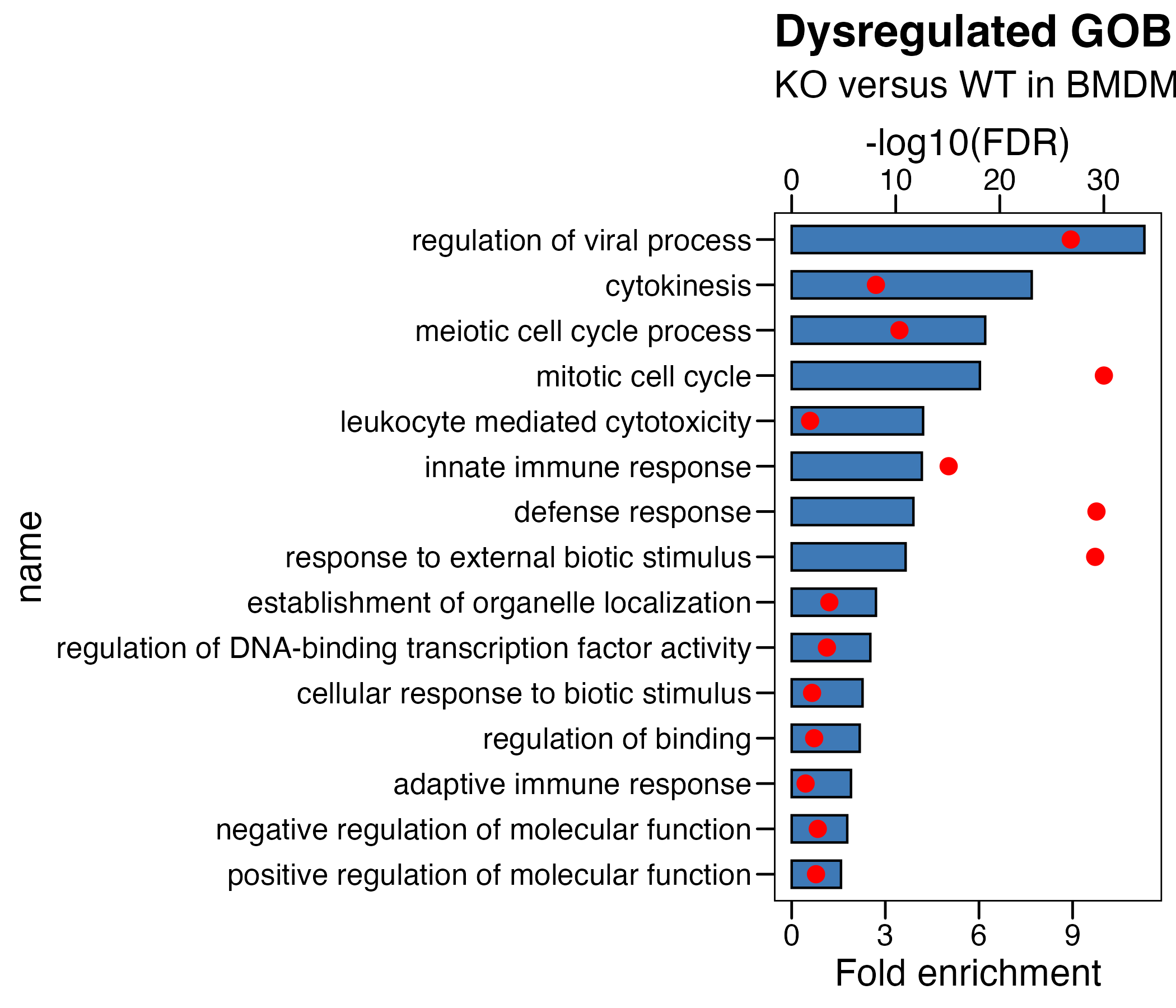
## (2) KO_WT in LPS
df <- read.xlsx("./data/7.BMDM-Enrichment_KO.LPS_WT.LPS.xlsx",sheet = 2)
df <- df %>% arrange(-fc) %>% mutate(name=factor(name,level=rev(name))) %>%
                  mutate(logFDR = -log10(adjp))  %>%
                  mutate(logFDR.plot = logFDR/2.5 ) # 将要画的第二个轴,先转换到第一个轴的范围内
# plot
p <- ggplot(df, aes(x=name )) +
          geom_col(aes(y=fc),fill = "#3e79b6",color = "black",width = 0.6)  +
          theme_base() +
          coord_flip() +
          geom_point(aes(y=logFDR.plot),fill = "red",color = "red", size = 3)+
          scale_y_continuous(
              # Features of the first axis
              name = "Fold enrichment",
              # Add a second axis and specify its features
              sec.axis = sec_axis(~.*2.5, name="-log10(FDR)") # 将第二个轴,转换回原数据范围内
              )  +
              ggtitle(label = "Dysregulated GOBP",
                      subtitle = "KO.LPS versus WT.LPS in BMDM") +
              theme(plot.background = element_blank())
ggsave("./results/Figure1/Figure1_B_right.BMDM_KO_WT_LPS.pdf",p,width = 8,height = 6)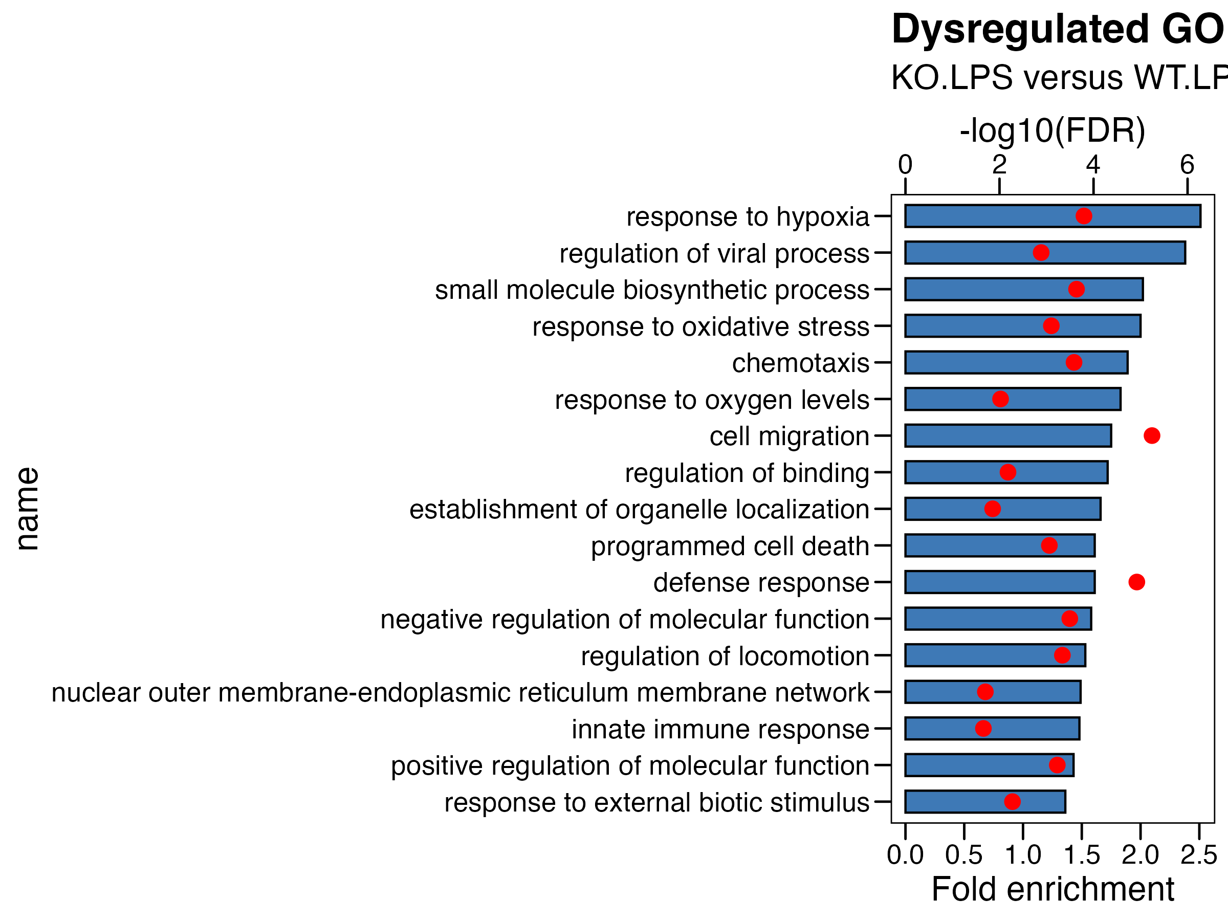
#----------------------------------------------------------------------------------
#  Step 4: KEGG analysis
#----------------------------------------------------------------------------------
## (1) KO_WT
# DE genes
deg_vec <- ls_limma[["KO_WT"]] %>% filter(group!="not sig") %>% pull(GeneSymbol) %>% unique()
# enrichment
esad <- oSEAadv(deg_vec, kegg, size.range=c(15,1500), test="fisher", min.overlap=3)  ## 最小3
df_eTerm.1 <- esad %>% oSEAextract() %>%
                  #filter(adjp<5e-2, distance==3) %>%
                  mutate(group=namespace) %>% group_by(group) %>%
                  arrange(group,adjp)

## (2) KO.LPS_WT.LPS
# DE genes
deg_vec <- ls_limma[["KO.LPS_WT.LPS"]] %>% filter(group!="not sig") %>% pull(GeneSymbol) %>% unique()
# enrichment
esad <- oSEAadv(deg_vec, kegg, size.range=c(15,1500), test="fisher", min.overlap=3)
df_eTerm.2 <- esad %>% oSEAextract() %>%
                  #filter(adjp<5e-2, distance==3) %>%
                  mutate(group=namespace) %>% group_by(group) %>%
                  arrange(group,adjp)
# output
ls_eTerm <- list(KO_WT=df_eTerm.1,
                 KO.LPS_WT.LPS=df_eTerm.2)
ls_eTerm %>% openxlsx::write.xlsx("./results/Figure1/BMDM_KEGG_KO_WT.xlsx")