2 Figure S4
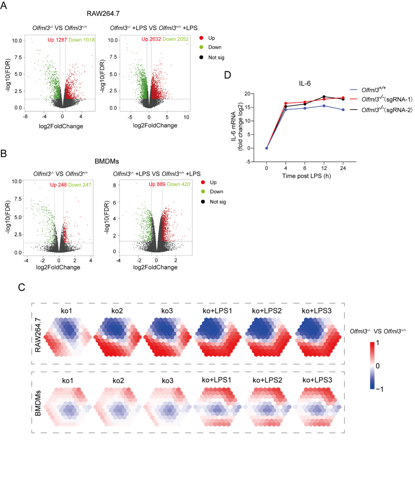
Figure S4. Analyses of the effects of Olfml3 knockout at the transcriptional level. (A-B) RNA-Seq analyses of the effects of Olfml3 knockout on gene expression in RAW264.7 (A) and BMDMs (B) in the absence and presence of LPS stimulation. The RNA-Seq data are from three biological replicates. DEGs with adjusted p value < 0.05 and fold change > 1.5 are highlighted in red (upregulation) and green (downregulation). (C) Self-organizing learning map of illustrating sample-specific expression profiles. Illustrations are displayed for samples separately derived from s in RAW264.7 (top panel) and BMDMs (bottom panel) cell lines, with colors indicating fold change relative to the wildtypes. (D) Analysis of the effects of Olfml3 knockout on IL-6 mRNA expression in RAW264.7 cells in response to LPS stimulation.
2.1 (A) DEGs in RAW264.7
# BiocManager::install("hfang-bristol/PIONE", dependencies=T)
# BiocManager::install("hfang-bristol/XGR", dependencies=T)
library(gmodels)
library(tidyr)
library(ggpubr)
library(ggthemes)
library(patchwork)
library(limma)
library(PIONE)
library(tidyverse)
library(XGR)
dir.create("./results/FigureS4/",recursive = T)
#----------------------------------------------------------------------------------
#  Step 1: Load the Data
#----------------------------------------------------------------------------------
rna  <- readRDS("./data/20231014_Oldml3_RAW_rna.rds")
meta <- readRDS("./data/20231014_Oldml3_RAW_meta.rds")
info <- readRDS("./data/20231014_Oldml3_RNA_info.rds")
#----------------------------------------------------------------------------------
#  Step 2: DEG
#----------------------------------------------------------------------------------
identical(meta$ID,colnames(rna))
## log 2 FPKM
rna <- log2(rna+0.1)
## limma
meta$contrast <- as.factor(meta$Type)
design    <- model.matrix(~ 0 + contrast  , data = meta)
fit       <- lmFit(rna, design)
contrast  <- makeContrasts( KO_WT = contrastko - contrastwt ,
                            KO.LPS_WT.LPS = contrastko_lps - contrastwt_lps,
                            levels = design)
fits      <- contrasts.fit(fit, contrast)
ebFit     <- eBayes(fits)
## result
# KO_WT
limma.res.1 <- topTable(ebFit, coef = "KO_WT", adjust.method = 'fdr', number = Inf)
limma.res.1 <- limma.res.1 %>% filter(!is.na(adj.P.Val)) %>%
              mutate( logP = -log10(P.Value) ) %>%
              mutate( contrast = "KO_WT") %>%
              mutate( cellline = "RAW") %>%
              mutate( ID = rownames(limma.res.1)) %>%
              mutate( logFDR = -log10(adj.P.Val) ) %>%
              as_tibble() %>%
              left_join(info,by=c('ID'='gene_id')) %>%
              dplyr::select(GeneSymbol,everything())
limma.res.1 <- limma.res.1 %>% mutate(group = case_when( adj.P.Val<0.05&logFC>0.58 ~ "up",
                                                         adj.P.Val<0.05&logFC< -0.58 ~ "down",
                                                         .default = "not sig"))
limma.res.1 %>% dplyr::count(group) # UP:1287 ; DOWN:1018 ; not:24435
# KO.LPS_WT.LPS
limma.res.2 <- topTable(ebFit, coef = "KO.LPS_WT.LPS", adjust.method = 'fdr', number = Inf)
limma.res.2 <- limma.res.2 %>% filter(!is.na(adj.P.Val)) %>%
              mutate( logP = -log10(P.Value) ) %>%
              mutate( contrast = "KO.LPS_WT.LPS") %>%
              mutate( cellline = "RAW") %>%
              mutate( ID = rownames(limma.res.2)) %>%
              mutate( logFDR = -log10(adj.P.Val) ) %>%
              as_tibble() %>%
              left_join(info,by=c('ID'='gene_id')) %>%
              dplyr::select(GeneSymbol,everything())
limma.res.2 <- limma.res.2 %>% mutate(group = case_when( adj.P.Val<0.05&logFC>0.58 ~ "up",
                                                         adj.P.Val<0.05&logFC< -0.58 ~ "down",
                                                         .default = "not sig"))
limma.res.2 %>% dplyr::count(group) # UP:2632 ; DOWN:2052 ; not:22056
# combine results
ls_limma <- list(KO_WT=limma.res.1,
                 KO.LPS_WT.LPS=limma.res.2)
## output
write.xlsx( ls_limma, "./results/FigureS4/FigureS4_A.Limma_fdr0.05_fc1.5.xlsx", overwrite = T, rowNames = F)
saveRDS(ls_limma,"./results/FigureS4/FigureS4_A.Limma_fdr0.05_fc1.5.rds")
#----------------------------------------------------------------------------------
#  Step 3: Volcano
#----------------------------------------------------------------------------------
## volcano
# KO_WT
pdata <- limma.res.1 %>% mutate(group=factor(group,levels = c("up","down","not sig")),
                                label=ifelse(group!="not sig",GeneSymbol,""))
my_label <- paste0( "Cutoff:FDR<0.05 & [FC]>1.5 ; \n" , "Up:",table(pdata$group)[1]," ; " ,"Down:" , table(pdata$group)[2])
# label top 20 sig genes
degs.1 <- ls_limma[[1]] %>% arrange(P.Value) %>% filter(group=="up") %>% dplyr::slice(1:20) %>% pull(ID)
degs.2 <- ls_limma[[1]] %>% arrange(P.Value) %>% filter(group=="down") %>% dplyr::slice(1:20) %>% pull(ID)
pdata <- pdata %>% mutate(label=case_when(ID %in% c(degs.1,degs.2) ~ GeneSymbol,
                                          .default = ""))
p <- ggscatter(pdata,
                 x = "logFC", y = "logFDR",
                 color = "group", size = 1,
                 main = paste0("KO_WT in RAW") ,
                 xlab = "log2FoldChange", ylab = "-log10(FDR)",
                 palette = c("#CC0000","#339900","#444444"),
                 #label = pdata$label,font.label = 10, repel = T,
                 xlim = c(-10, 10)
               )+
    theme_base()+
    geom_hline(yintercept = -log10(0.05), linetype="dashed", color = "#222222") +
    geom_vline(xintercept = log2(1.5) , linetype="dashed", color = "#222222")+
    geom_vline(xintercept = -log2(1.5) , linetype="dashed", color = "#222222")+
    labs(subtitle = my_label) +
    theme(plot.background = element_blank())
ggsave("./results/FigureS4/FigureS4_A_left.Volcano.pdf", p, width = 8, height = 8)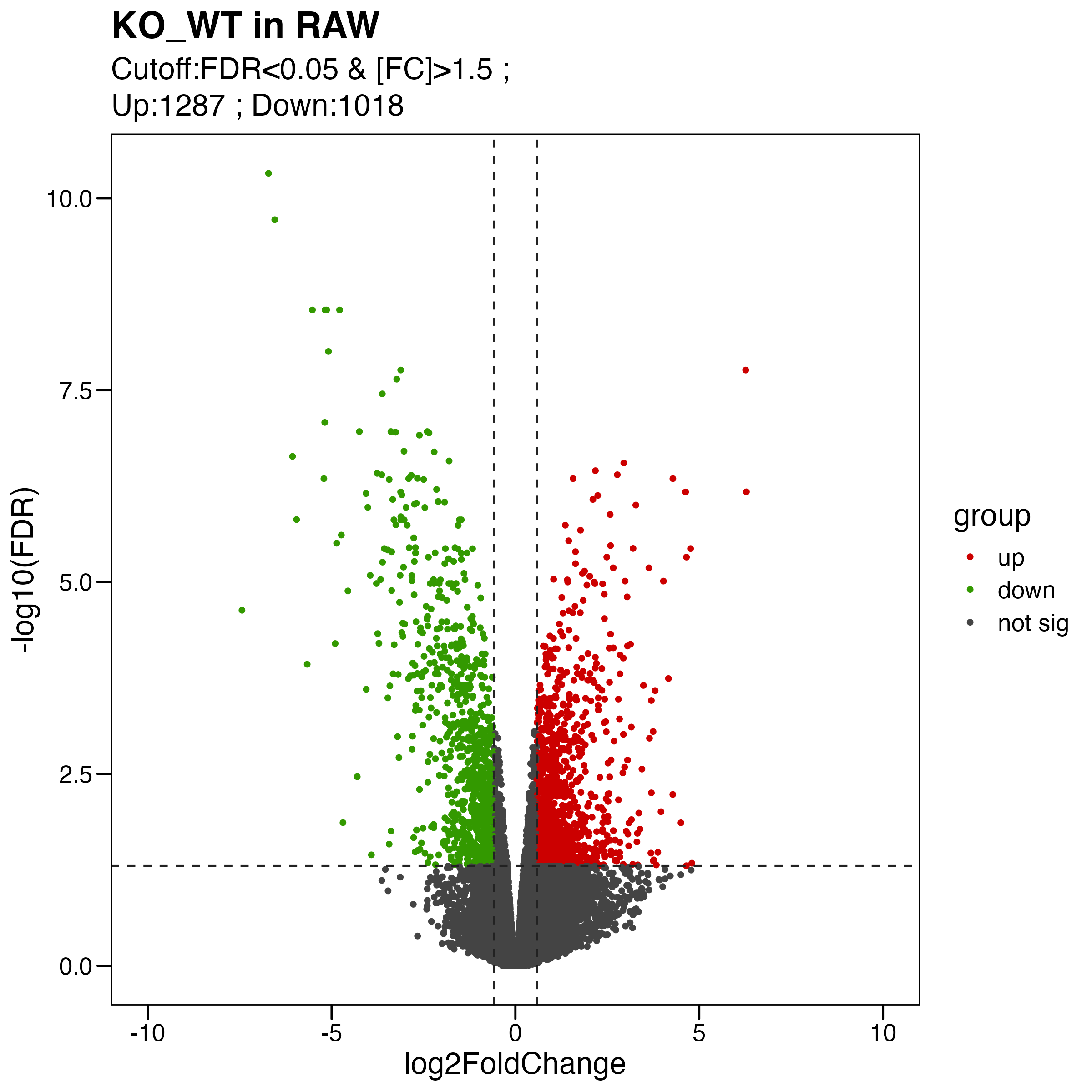
# KO.LPS_WT.LPS
pdata <- limma.res.2 %>% mutate(group=factor(group,levels = c("up","down","not sig")),
                                label=ifelse(group!="not sig",GeneSymbol,""))
my_label <- paste0( "Cutoff:FDR<0.05 & [FC]>1.5 ; \n" , "Up:",table(pdata$group)[1]," ; " ,"Down:" , table(pdata$group)[2])
# label top 20 sig genes
degs.1 <- ls_limma[[2]] %>% arrange(P.Value) %>% filter(group=="up") %>% dplyr:: slice(1:20) %>% pull(ID)
degs.2 <- ls_limma[[2]] %>% arrange(P.Value) %>% filter(group=="down") %>% dplyr:: slice(1:20) %>% pull(ID)
pdata <- pdata %>% mutate(label=case_when(ID %in% c(degs.1,degs.2) ~ GeneSymbol,
                                          .default = ""))
p <- ggscatter(pdata,
                 x = "logFC", y = "logFDR",
                 color = "group", size = 1,
                 main = paste0("KO.LPS_WT.LPS in RAW") ,
                 xlab = "log2FoldChange", ylab = "-log10(FDR)",
                 palette = c("#CC0000","#339900","#444444"),
                 #label = pdata$label,font.label = 10, repel = T,
                 xlim = c(-10,10)
               )+
    theme_base()+
    geom_hline(yintercept = -log10(0.05), linetype="dashed", color = "#222222") +
    geom_vline(xintercept = log2(1.5) , linetype="dashed", color = "#222222")+
    geom_vline(xintercept = -log2(1.5) , linetype="dashed", color = "#222222")+
    labs(subtitle = my_label) + theme(plot.background = element_blank())
ggsave("./results/FigureS4/FigureS4_A_right.Volcano.pdf", p, width = 8, height = 8)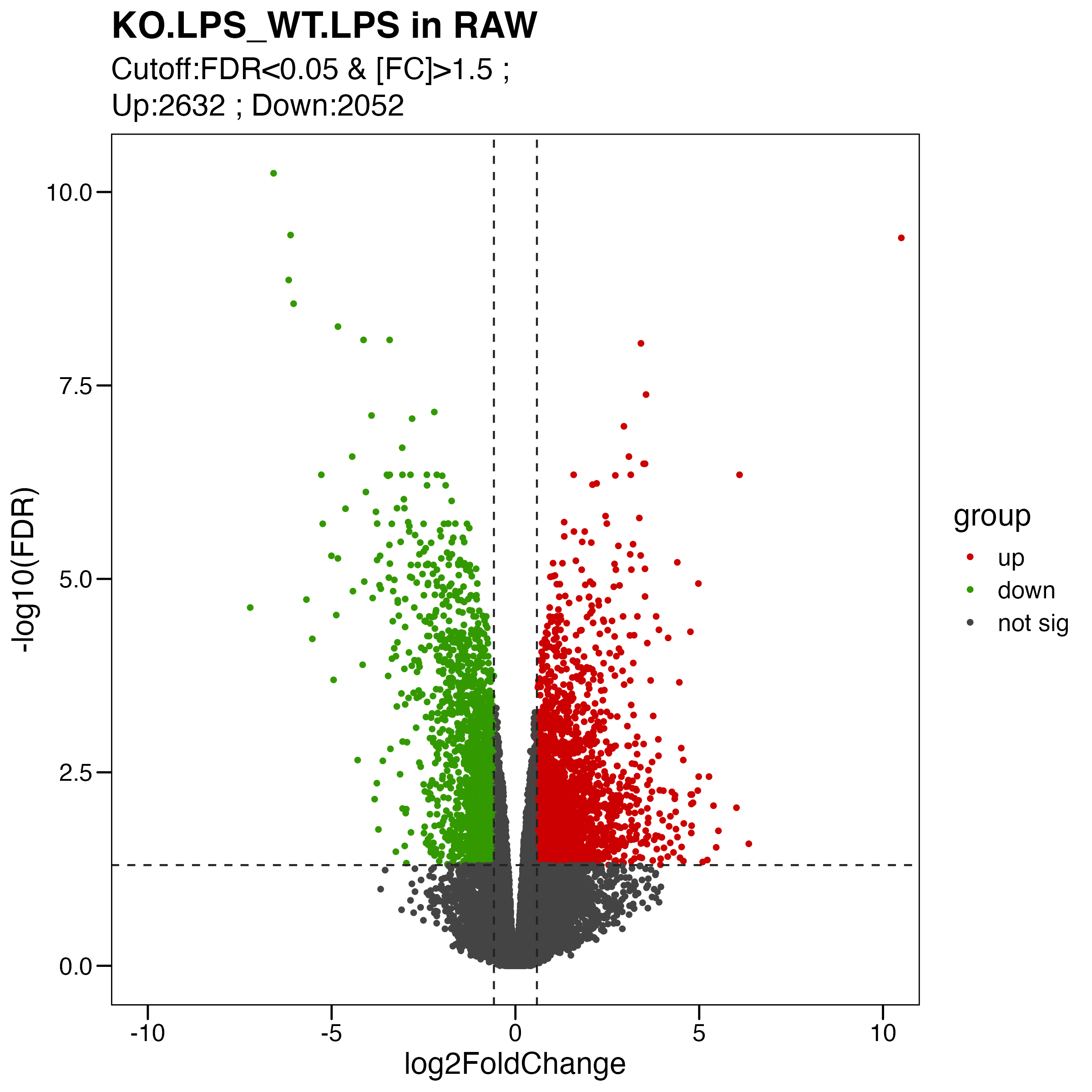
2.2 (B) DEGs in BMDMs
library(gmodels)
library(tidyr)
library(ggpubr)
library(ggthemes)
library(patchwork)
library(limma)
library(PIONE)
library(tidyverse)
library(XGR)
#----------------------------------------------------------------------------------
#  Step 1: Load the Data
#----------------------------------------------------------------------------------
rna  <- readRDS("./data/20231014_Oldml3_BMDM_rna.rds")
meta <- readRDS("./data/20231014_Oldml3_BMDM_meta.rds")
info <- readRDS("./data/20231014_Oldml3_RNA_info.rds")
#----------------------------------------------------------------------------------
#  Step 2: DEG
#----------------------------------------------------------------------------------
identical(rownames(meta),colnames(rna))
## log 2 FPKM
rna <- log2(rna+0.1)
## limma
meta$contrast <- as.factor(meta$Type)
design    <- model.matrix(~ 0 + contrast  , data = meta)
fit       <- lmFit(rna, design)
contrast  <- makeContrasts( KO_WT = contrastko - contrastwt ,
                            KO.LPS_WT.LPS = contrastko_lps - contrastwt_lps,
                            levels = design)
fits      <- contrasts.fit(fit, contrast)
ebFit     <- eBayes(fits)
## result
# KO_WT
limma.res.1 <- topTable(ebFit, coef = "KO_WT", adjust.method = 'fdr', number = Inf)
limma.res.1 <- limma.res.1 %>% filter(!is.na(adj.P.Val)) %>%
              mutate( logP = -log10(P.Value) ) %>%
              mutate( contrast = "KO_WT") %>%
              mutate( cellline = "BMDM") %>%
              mutate( ID = rownames(limma.res.1)) %>%
              mutate( logFDR = -log10(adj.P.Val) ) %>%
              as_tibble() %>%
              left_join(info,by=c('ID'='gene_id')) %>%
              dplyr::select(GeneSymbol,everything())
limma.res.1 <- limma.res.1 %>% mutate(group = case_when( adj.P.Val<0.05&logFC>0.58 ~ "up",
                                                         adj.P.Val<0.05&logFC< -0.58 ~ "down",
                                                         .default = "not sig"))
limma.res.1 %>% dplyr::count(group)
# KO.LPS_WT.LPS
limma.res.2 <- topTable(ebFit, coef = "KO.LPS_WT.LPS", adjust.method = 'fdr', number = Inf)
limma.res.2 <- limma.res.2 %>% filter(!is.na(adj.P.Val)) %>%
              mutate( logP = -log10(P.Value) ) %>%
              mutate( contrast = "KO.LPS_WT.LPS") %>%
              mutate( cellline = "BMDM") %>%
              mutate( ID = rownames(limma.res.2)) %>%
              mutate( logFDR = -log10(adj.P.Val) ) %>%
              as_tibble() %>%
              left_join(info,by=c('ID'='gene_id')) %>%
              dplyr::select(GeneSymbol,everything())
limma.res.2 <- limma.res.2 %>% mutate(group = case_when( adj.P.Val<0.05&logFC>0.58 ~ "up",
                                                         adj.P.Val<0.05&logFC< -0.58 ~ "down",
                                                         .default = "not sig"))
limma.res.2 %>% dplyr::count(group)
# combine results
ls_limma <- list(KO_WT=limma.res.1,
                 KO.LPS_WT.LPS=limma.res.2)
## output
write.xlsx( ls_limma, "./results/FigureS4/FigureS4_B.Limma_fdr0.05_fc1.5.xlsx", overwrite = T, rowNames = F)
saveRDS(ls_limma,"./results/FigureS4/FigureS4_B.Limma_fdr0.05_fc1.5.rds")
#----------------------------------------------------------------------------------
#  Step 3: Volcano
#----------------------------------------------------------------------------------
## volcano
# KO_WT
pdata <- limma.res.1 %>% mutate(group=factor(group,levels = c("up","down","not sig")),
                                label=ifelse(group!="not sig",GeneSymbol,""))
my_label <- paste0( "Cutoff:FDR<0.05 & [FC]>1.5 ; \n" , "Up:",table(pdata$group)[1]," ; " ,"Down:" , table(pdata$group)[2])
# label top 20 sig genes
degs.1 <- ls_limma[[1]] %>% arrange(P.Value) %>% filter(group=="up") %>%  dplyr::slice(1:20) %>% pull(ID)
degs.2 <- ls_limma[[1]] %>% arrange(P.Value) %>% filter(group=="down") %>% dplyr::slice(1:20) %>% pull(ID)
pdata <- pdata %>% mutate(label=case_when(ID %in% c(degs.1,degs.2) ~ GeneSymbol,
                                          .default = ""))
p <- ggscatter(pdata,
                 x = "logFC", y = "logFDR",
                 color = "group", size = 1,
                 main = paste0("KO_WT in BMDM") ,
                 xlab = "log2FoldChange", ylab = "-log10(FDR)",
                 palette = c("#CC0000","#339900","#444444"),
                 #label = pdata$label,font.label = 10, repel = T,
                 xlim = c(-5,5)
               )+
    theme_base()+
    geom_hline(yintercept = -log10(0.05), linetype="dashed", color = "#222222") +
    geom_vline(xintercept = log2(1.5) , linetype="dashed", color = "#222222")+
    geom_vline(xintercept = -log2(1.5) , linetype="dashed", color = "#222222")+
    labs(subtitle = my_label) + theme(plot.background = element_blank())
ggsave("./results/FigureS4/FigureS4_B_left.Volcano.pdf", p, width = 8, height = 8)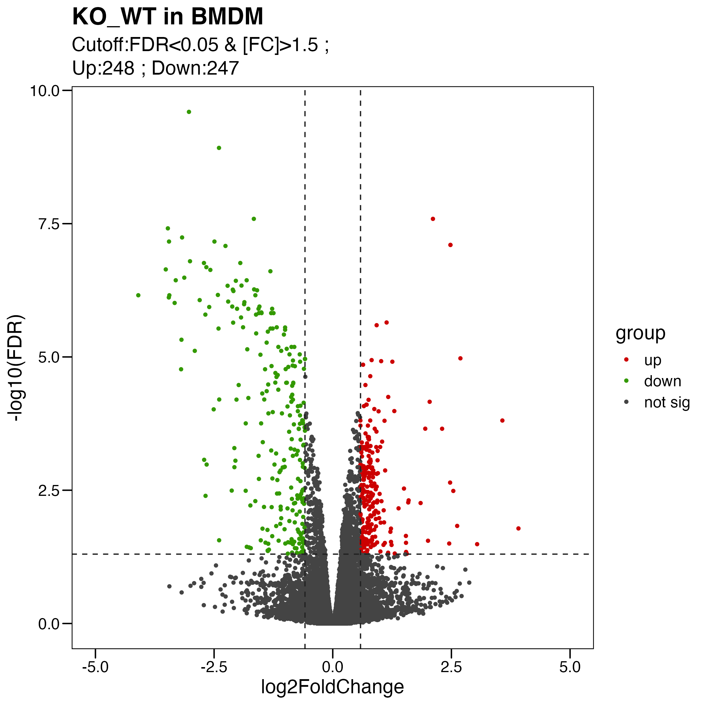
# KO.LPS_WT.LPS
pdata <- limma.res.2 %>% mutate(group=factor(group,levels = c("up","down","not sig")),
                                label=ifelse(group!="not sig",GeneSymbol,""))
my_label <- paste0( "Cutoff:FDR<0.05 & [FC]>1.5 ; \n" , "Up:",table(pdata$group)[1]," ; " ,"Down:" , table(pdata$group)[2])
# label top 20 sig genes
degs.1 <- ls_limma[[2]] %>% arrange(P.Value) %>% filter(group=="up") %>% dplyr::slice(1:20) %>% pull(ID)
degs.2 <- ls_limma[[2]] %>% arrange(P.Value) %>% filter(group=="down") %>%  dplyr::slice(1:20) %>% pull(ID)
pdata <- pdata %>% mutate(label=case_when(ID %in% c(degs.1,degs.2) ~ GeneSymbol,
                                          .default = ""))
p <- ggscatter(pdata,
                 x = "logFC", y = "logFDR",
                 color = "group", size = 1,
                 main = paste0("KO.LPS_WT.LPS in BMDM") ,
                 xlab = "log2FoldChange", ylab = "-log10(FDR)",
                 palette = c("#CC0000","#339900","#444444"),
                 #label = pdata$label,font.label = 10, repel = T,
                 xlim = c(-5,5)
               )+
    theme_base()+
    geom_hline(yintercept = -log10(0.05), linetype="dashed", color = "#222222") +
    geom_vline(xintercept = log2(1.5) , linetype="dashed", color = "#222222")+
    geom_vline(xintercept = -log2(1.5) , linetype="dashed", color = "#222222")+
    labs(subtitle = my_label) + theme(plot.background = element_blank())
ggsave("./results/FigureS4/FigureS4_B_right.Volcano.pdf", p, width = 8, height = 8)
2.3 (C) Self-organizing map
library(supraHex)
#----------------------------------------------------------------------------------
#  Step 1: Load the Data
#----------------------------------------------------------------------------------
## cellline: raw
rna  <- readRDS("./data/20231014_Oldml3_RAW_rna.rds")
rna <- log2(rna+0.1)
info <- readRDS("./data/20231014_Oldml3_RNA_info.rds")
ls_limma <- readRDS("./results/FigureS4/FigureS4_A.Limma_fdr0.05_fc1.5.rds")
# union DEGs
degs.1 <- do.call(rbind,ls_limma) %>% filter(group != "not sig")
# DEGs matrix
degs.matrix <- rna[,c("d1","d2","d3","O1","O2","O3","dL1","dL2","dL3","OL1","OL2","OL3")]
degs.matrix <- degs.matrix %>% rownames_to_column("ID") %>%
                  left_join(info,by = c('ID'='gene_id')) %>%
                  dplyr::select(-ID) %>%
                  distinct(GeneSymbol,.keep_all = T) %>%
                  filter(!is.na(GeneSymbol)) %>%
                  filter(GeneSymbol!="-") %>%
                  column_to_rownames(var = "GeneSymbol") # 5291 genes
colnames(degs.matrix) <- c("wt1","wt2","wt3","ko1","ko2","ko3",
                           "wtl1","wtl2","wtl3","kol1","kol2","kol3")
#           wt1   wt2  wt3 ko1 ko2 ko3 wtl1 wtl2 wtl3 kol1 kol2 kol3
# Eif2s3y 10.87 10.51 9.89   0   0   0 9.48 9.92 9.00    0    0    0
# Psma8   10.21  8.82 8.78   0   0   0 6.67 6.46 7.42    0    0    0
# Ddx3y    5.00  4.64 3.92   0   0   0 7.29 6.30 7.75    0    0    0
# Tox2     3.21  3.44 3.62   0   0   0 0.16 0.10 0.12    0    0    0

# fold change matirx
wt.mean <- degs.matrix[,c("wt1","wt2","wt3")] %>% rowMeans()
wtl.mean <- degs.matrix[,c("wtl1","wtl2","wtl3")] %>% rowMeans()

ko.data <- degs.matrix[,c("ko1","ko2","ko3")] - wt.mean # fold change
kol.data <- degs.matrix[,c("kol1","kol2","kol3")] - wtl.mean

data <- cbind(ko.data,kol.data)
data.raw <- data

## cellline:bmdm
rna  <- readRDS("./data/20231014_Oldml3_BMDM_rna.rds")
rna <- log2(rna+0.1)
info <- readRDS("./data/20231014_Oldml3_RNA_info.rds")
ls_limma <- readRDS("./results/FigureS4/FigureS4_B.Limma_fdr0.05_fc1.5.rds")
# union DEGs
degs.2 <- do.call(rbind,ls_limma) %>% filter(group != "not sig")
degs.matrix <- rna[,c("WT1","WT2","WT3","KO1","KO2","KO3",
                             "WL1","WL2","WL3","KL1","KL2","KL3")]
degs.matrix <- degs.matrix %>% rownames_to_column("ID") %>%
                  left_join(info,by = c('ID'='gene_id')) %>%
                  dplyr::select(-ID) %>%
                  distinct(GeneSymbol,.keep_all = T) %>%
                  filter(!is.na(GeneSymbol)) %>%
                  filter(GeneSymbol!="-") %>%
                  column_to_rownames(var = "GeneSymbol") # 1586 genes
colnames(degs.matrix) <- c("wt1","wt2","wt3","ko1","ko2","ko3",
                           "wtl1","wtl2","wtl3","kol1","kol2","kol3")
# fold change matirx
wt.mean <- degs.matrix[,c("wt1","wt2","wt3")] %>% rowMeans()
wtl.mean <- degs.matrix[,c("wtl1","wtl2","wtl3")] %>% rowMeans()

ko.data <- degs.matrix[,c("ko1","ko2","ko3")] - wt.mean # fold change
kol.data <- degs.matrix[,c("kol1","kol2","kol3")] - wtl.mean

data <- cbind(ko.data,kol.data)
data.bmdm <- data

## merge 2 matrix
colnames(data.bmdm) <- paste0(colnames(data.bmdm),"_bmdm")
colnames(data.raw) <- paste0(colnames(data.raw),"_raw")
DEgenes <- union(degs.1$GeneSymbol,degs.2$GeneSymbol) %>% unique()
DEgenes <- intersect(intersect(DEgenes,rownames(data.bmdm)),intersect(DEgenes,rownames(data.raw)))# 6163 genes
data.bmdm <- data.bmdm[DEgenes,]
data.raw <- data.raw[DEgenes,]
identical(rownames(data.bmdm),rownames(data.raw))
data <- cbind(data.raw,data.bmdm) # 6163 genens * 12 samples

#----------------------------------------------------------------------------------
#  Step 2: SupraHex
#----------------------------------------------------------------------------------
# Train the supra-hexagonal map with input data only
sMap <- sPipeline(data=data,shape = "suprahex",scaling = 1, finetuneSustain = T)
# overlay additional data onto the trained map
sOverlay <- sMapOverlay(sMap=sMap, data=data, additional=data)
# viewing the distribution of that additional data
pdf("./results/FigureS4/FigureS4_C_DEGs_supraHex.pdf",height = 4,width = 8)
visHexMulComp(sOverlay, zlim=c(-1,1),
              title.rotate = 0,newpage = F,rect.grid=c(1,6))
dev.off()
# Perform partitioning operation on the map to obtain continuous clusters
sBase <- sDmatCluster(sMap)
pdf("./results/FigureS4/FigureS4_C_DEGs_supraHex_Cluster.pdf",height = 5,width = 4)
visDmatCluster(sMap, sBase,newpage = F,border.color = "lightgrey",
               gp = grid::gpar(cex = 1.5, font = 2, col = "black"),
               colormap = c("rainbow"),
)
dev.off()
# output
sWriteData(sMap,data, sBase,
           filename="./results/FigureS4/FigureS4_C_DEGs_supraHex_Cluster.csv",
           keep.data =T)