5 Figure 4

Figure 4: Metabolic information yields an independent prognostic clustering classification for BCP-ALL and T-ALL.
A. The schematic workflow following SNF integration analysis. The BMMC omics data were inputted to generate a fused similarity network, which was subsequently utilized for sample clustering in this study.
B. The discrimination of three BCP-ALL clusters (BC1, BC2 and BC3) generated from SNF method.
C. The association of the three metabolic clusters with clinical OS in 75 BCP-ALL patients.
D. The multivariate Cox analysis reveals that the metabolic cluster bore an independent prognostic value for OS and EFS, respectively. The WBC was stratified by 30×109/L. In the genetic-based risk stratification, BCR::ABL1, ETV6::RUNX1, DUX4::IGH and TCF3::PBX1 were categorized into standard risk subgroup, otherwise were into poor risk subgroup.
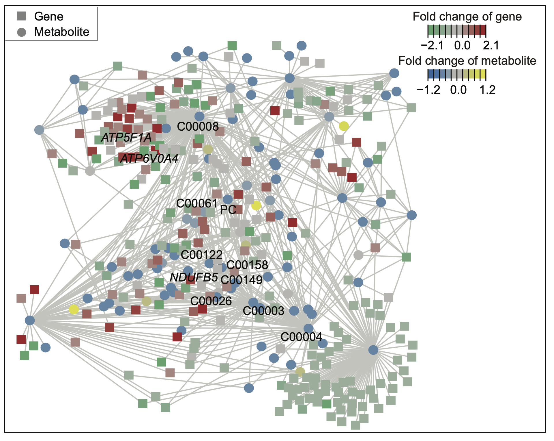
E. A core metabolism-based subnetwork that best explains the difference between BC3 and BC1/2. In this network, each circular node represents a metabolite, labeled with its KEGG ID, and each square node represents a gene. Node colors indicate logFC values: red and green signify different gene expression levels, while yellow and blue signify varying metabolite levels. The highlighted labels correspond to pathways in the cholesterol metabolism and nicotinate and nicotinamide metabolism.
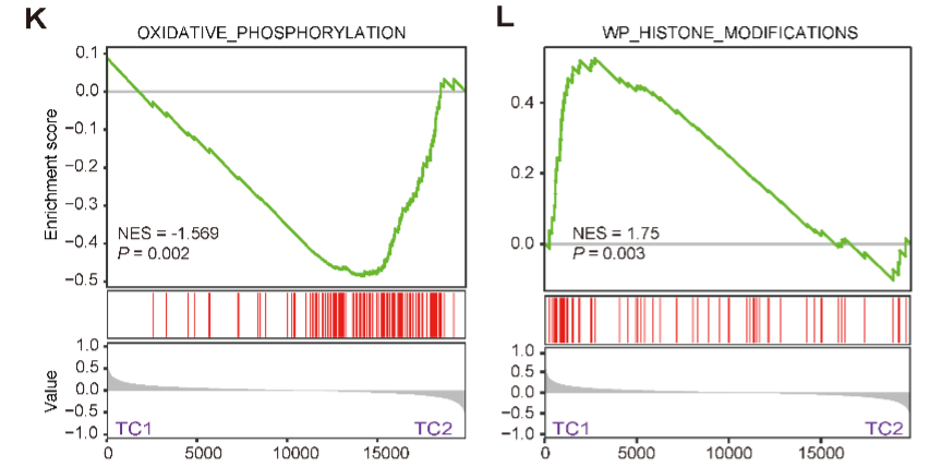
F. The discrimination of two T-ALL clusters (TC1 and TC2) based on SNF method.
G. The association of the two metabolic clusters with clinical OS outcomes in 24 T-ALL patients. The result suggested TC1 was of significantly poorer prognosis than TC2.
H. A core metabolism-based subnetwork that best explains the difference between TC2 and TC1. The highlighted labels correspond to pathways in the TCA and OXPHOS. PC refers to a group of phosphatidylcholines without specific KEGG IDs.
5.1 (A) Schematic Workflow
The schematic workflow following integrated analysis. The BMMC omics data are inputted to generate a fused similarity network, which is subsequently utilized for sample clustering in this study.
library(dplyr)
library(MNet)
library(survival)
library(survminer)

#-------------------------------------------------------------------------------
#  Step 1: Cox regression of metabolomics of BCP-ALL
#-------------------------------------------------------------------------------
sample_info <- readxl::read_excel("raw_data/sample_clinical_201_info.xlsx") %>%
  as.data.frame() %>%
  dplyr::filter(!is.na(METc_BM_D0_ID)) %>%
  dplyr::filter(Lineage=="B") %>%
  dplyr::mutate(bianhao=gsub("RJ-","A",Pid)) %>%
  dplyr::select(bianhao,METc_BM_D0_ID)

dat_cell <- data.table::fread("raw_data/cell_dat_final_reuslt_v0329.txt") %>%
  as.data.frame() %>%
  tibble::column_to_rownames("label") %>%
  dplyr::select(all_of(sample_info$METc_BM_D0_ID)) %>%
  log1p()
names(dat_cell) <- sample_info$bianhao

clinical <- readxl::read_excel("raw_data/08 队列病人生存资料-v231026.xlsx") %>%
  as.data.frame() %>%
  dplyr::select(bianhao,OS_stat,OS) %>%
  dplyr::inner_join(sample_info,by=c("bianhao")) %>%
  dplyr::arrange(match(bianhao,sample_info$bianhao)) %>%
  dplyr::select(-METc_BM_D0_ID) %>%
  unique()

dat_t <- t(dat_cell) %>%
  data.frame() %>%
  tibble::rownames_to_column(var="bianhao") %>%
  dplyr::left_join(clinical,by="bianhao") %>%
  dplyr::select(OS,OS_stat,everything()) %>%
  tibble::column_to_rownames("bianhao") %>%
  dplyr::rename("time"="OS") %>%
  dplyr::rename("status"="OS_stat")
metabolite_name <- names(dat_t)[3:ncol(dat_t)]

dat_t_raw <- t(dat_cell) %>%
  as.data.frame() %>%
  tibble::rownames_to_column(var="bianhao") %>%
  dplyr::left_join(clinical,by="bianhao") %>%
  dplyr::select(OS,OS_stat,everything()) %>%
  tibble::column_to_rownames("bianhao") %>%
  dplyr::rename("time"="OS") %>%
  dplyr::rename("status"="OS_stat")
metabolite_name_raw <- names(dat_t_raw)[3:ncol(dat_t_raw)]
dd <- data.frame(name=metabolite_name,name_raw=metabolite_name_raw)

univ_formulas <- lapply(metabolite_name,function(x) stats::as.formula(paste('survival::Surv(time, status)~', x)))

univ_models <- lapply( univ_formulas, function(x){survival::coxph(x, data = dat_t)})

univ_results <- lapply(univ_models,
                       function(x){
                         x <- summary(x)
                         p.value<-signif(x$wald["pvalue"], digits=2)
                         wald.test<-signif(x$wald["test"], digits=2)
                         beta<-signif(x$coef[1], digits=2);#coeficient beta
                         HR <-signif(x$coef[2], digits=2);#exp(beta)
                         HR.confint.lower <- signif(x$conf.int[,"lower .95"], 2)
                         HR.confint.upper <- signif(x$conf.int[,"upper .95"],2)
                         HR <- paste0(HR, " (",
                                      HR.confint.lower, "-", HR.confint.upper, ")")
                         name <- rownames(x$coefficients)
                         res<-c(name,beta, HR, wald.test, p.value)
                         names(res)<-c("name","beta", "HR (95% CI for HR)", "wald.test","p.value")
                         return(res)
                       })
res <- t(as.data.frame(univ_results, check.names = FALSE))
result <- as.data.frame(res)

metabolite_all <- result %>%
  dplyr::left_join(dd,by=c("name"))

write.table(metabolite_all,"result/Figure4/4A_1.cox_metabolite_all_B.txt",quote=F,row.names=F,sep="\t")

#-------------------------------------------------------------------------------
#  Step 2: Cox regression of  transcriptomics of BCP-ALL
#-------------------------------------------------------------------------------
gene_metabolite1 <- gene_metabolite %>% dplyr::filter(dest_type=="gene")
gene2 <- PathwayExtendData %>% filter(type=="gene")
gene_filter <- unique(c(gene_metabolite1$gene,gene2$name))
length(gene_filter)

sample_rna <- readxl::read_excel("raw_data/sample_clinical_201_info.xlsx") %>%
  as.data.frame() %>%
  dplyr::filter(Lineage=="B") %>%
  dplyr::filter(!is.na(RNA_ID)) %>%
  dplyr::mutate(bianhao=gsub("RJ-","A",Pid)) %>%
  dplyr::select(bianhao,RNA_id_raw)

dat_gene <- readRDS("raw_data/20231113_RNA_ALL_VST_coding.rds") %>%
  as.data.frame() %>%
  dplyr::select(sample_rna$RNA_id_raw) %>%
  tibble::rownames_to_column(var="label") %>%
  dplyr::filter(label %in% gene_filter) %>%
  tibble::column_to_rownames("label")

names(dat_gene) <- sample_rna$bianhao

dat_gene_0 <- rowSums(dat_gene==0)
dat_gene <- dat_gene %>%
  dplyr::mutate(num=dat_gene_0) %>%
  dplyr::filter(num < 0.5*ncol(dat_gene)) %>%
  dplyr::select(-num)

clinical <- readxl::read_excel("raw_data/08 队列病人生存资料-v231026.xlsx") %>%
  as.data.frame() %>%
  dplyr::select(bianhao_new,OS_stat,OS) %>%
  dplyr::mutate(bianhao=paste0("A",bianhao_new)) %>%
  dplyr::select(-bianhao_new) %>%
  unique()

dat_t <- t(dat_gene) %>%
  data.frame() %>%
  tibble::rownames_to_column(var="bianhao") %>%
  dplyr::left_join(clinical,by="bianhao") %>%
  dplyr::select(OS,OS_stat,everything()) %>%
  tibble::column_to_rownames("bianhao") %>%
  dplyr::rename("time"="OS") %>%
  dplyr::rename("status"="OS_stat")
gene_name <- names(dat_t)[3:ncol(dat_t)]

dat_t_raw <- t(dat_gene) %>%
  as.data.frame() %>%
  tibble::rownames_to_column(var="bianhao") %>%
  dplyr::left_join(clinical,by="bianhao") %>%
  dplyr::select(OS,OS_stat,everything()) %>%
  tibble::column_to_rownames("bianhao") %>%
  dplyr::rename("time"="OS") %>%
  dplyr::rename("status"="OS_stat")
gene_name_raw <- names(dat_t_raw)[3:ncol(dat_t_raw)]
dd <- data.frame(name=gene_name,name_raw=gene_name_raw)

univ_formulas <- lapply(gene_name,function(x) stats::as.formula(paste('survival::Surv(time, status)~', x)))

univ_models <- lapply(univ_formulas, function(x){survival::coxph(x, data = dat_t)})

univ_results <- lapply(univ_models,
                       function(x){
                         x <- summary(x)
                         p.value<-signif(x$wald["pvalue"], digits=2)
                         wald.test<-signif(x$wald["test"], digits=2)
                         beta<-signif(x$coef[1], digits=2);#coeficient beta
                         HR <-signif(x$coef[2], digits=2);#exp(beta)
                         HR.confint.lower <- signif(x$conf.int[,"lower .95"], 2)
                         HR.confint.upper <- signif(x$conf.int[,"upper .95"],2)
                         HR <- paste0(HR, " (",
                                      HR.confint.lower, "-", HR.confint.upper, ")")
                         name <- rownames(x$coefficients)
                         res<-c(name,beta, HR, wald.test, p.value)
                         names(res)<-c("name","beta", "HR (95% CI for HR)", "wald.test","p.value")
                         return(res)
                       })
res <- t(as.data.frame(univ_results, check.names = FALSE))
result <- as.data.frame(res)

gene_all <- result %>%
  dplyr::left_join(dd,by="name")

write.table(gene_all,"result/Figure4/4A_1.cox_gene_all_B.txt",quote=F,row.names=F,sep="\t")

#------------------------------------------------------------------------------
# Step 3: Cox regression of metabolomics of T-ALL
#------------------------------------------------------------------------------
sample_info <- readxl::read_excel("raw_data/sample_clinical_201_info.xlsx") %>%
  as.data.frame() %>%
  dplyr::filter(!is.na(METc_BM_D0_ID)) %>%
  dplyr::filter(Lineage=="T") %>%
  dplyr::mutate(bianhao=gsub("RJ-","A",Pid)) %>%
  dplyr::select(bianhao,METc_BM_D0_ID)

dat_cell <- data.table::fread("raw_data/cell_dat_final_reuslt_v0329.txt") %>%
  as.data.frame() %>%
  tibble::column_to_rownames("label") %>%
  dplyr::select(all_of(sample_info$METc_BM_D0_ID)) %>%
  log1p()
names(dat_cell) <- sample_info$bianhao

clinical <- readxl::read_excel("raw_data/08 队列病人生存资料-v231026.xlsx") %>%
  as.data.frame() %>%
  dplyr::select(bianhao,OS_stat,OS) %>%
  dplyr::inner_join(sample_info,by=c("bianhao")) %>%
  dplyr::arrange(match(bianhao,sample_info$bianhao)) %>%
  dplyr::select(-METc_BM_D0_ID) %>%
  unique()

dat_t <- t(dat_cell) %>%
  data.frame() %>%
  tibble::rownames_to_column(var="bianhao") %>%
  dplyr::left_join(clinical,by="bianhao") %>%
  dplyr::select(OS,OS_stat,everything()) %>%
  tibble::column_to_rownames("bianhao") %>%
  dplyr::rename("time"="OS") %>%
  dplyr::rename("status"="OS_stat")
metabolite_name <- names(dat_t)[3:ncol(dat_t)]

dat_t_raw <- t(dat_cell) %>%
  as.data.frame() %>%
  tibble::rownames_to_column(var="bianhao") %>%
  dplyr::left_join(clinical,by="bianhao") %>%
  dplyr::select(OS,OS_stat,everything()) %>%
  tibble::column_to_rownames("bianhao") %>%
  dplyr::rename("time"="OS") %>%
  dplyr::rename("status"="OS_stat")
metabolite_name_raw <- names(dat_t_raw)[3:ncol(dat_t_raw)]
dd <- data.frame(name=metabolite_name,name_raw=metabolite_name_raw)

univ_formulas <- lapply(metabolite_name,function(x) stats::as.formula(paste('survival::Surv(time, status)~', x)))

univ_models <- lapply( univ_formulas, function(x){survival::coxph(x, data = dat_t)})

univ_results <- lapply(univ_models,
                       function(x){
                         x <- summary(x)
                         p.value<-signif(x$wald["pvalue"], digits=2)
                         wald.test<-signif(x$wald["test"], digits=2)
                         beta<-signif(x$coef[1], digits=2);
                         HR <-signif(x$coef[2], digits=2);
                         HR.confint.lower <- signif(x$conf.int[,"lower .95"], 2)
                         HR.confint.upper <- signif(x$conf.int[,"upper .95"],2)
                         HR <- paste0(HR, " (",
                                      HR.confint.lower, "-", HR.confint.upper, ")")
                         name <- rownames(x$coefficients)
                         res<-c(name,beta, HR, wald.test, p.value)
                         names(res)<-c("name","beta", "HR (95% CI for HR)", "wald.test","p.value")
                         return(res)
                       })
res <- t(as.data.frame(univ_results, check.names = FALSE))
result <- as.data.frame(res)

metabolite_all <- result %>%
  dplyr::left_join(dd,by=c("name"))

write.table(metabolite_all,"result/Figure4/4A_1.cox_metabolite_all_T.txt",quote=F,row.names=F,sep="\t")

#-------------------------------------------------------------------------------
#  Step 4: Cox regression of  transcriptomics of T-ALL
#-------------------------------------------------------------------------------
gene_metabolite1 <- gene_metabolite %>% dplyr::filter(dest_type=="gene")
gene2 <- PathwayExtendData %>% filter(type=="gene")
gene_filter <- unique(c(gene_metabolite1$gene,gene2$name))
length(gene_filter)

sample_rna <- readxl::read_excel("raw_data/sample_clinical_201_info.xlsx") %>%
  as.data.frame() %>%
  dplyr::filter(Lineage=="T") %>%
  dplyr::filter(!is.na(RNA_ID)) %>%
  dplyr::mutate(bianhao=gsub("RJ-","A",Pid)) %>%
  dplyr::select(bianhao,RNA_id_raw)

dat_gene <- readRDS("raw_data/20231113_RNA_ALL_VST_coding.rds") %>%
  as.data.frame() %>%
  dplyr::select(sample_rna$RNA_id_raw) %>%
  tibble::rownames_to_column(var="label") %>%
  dplyr::filter(label %in% gene_filter) %>%
  tibble::column_to_rownames("label")

names(dat_gene) <- sample_rna$bianhao

dat_gene_0 <- rowSums(dat_gene==0)
dat_gene <- dat_gene %>%
  dplyr::mutate(num=dat_gene_0) %>%
  dplyr::filter(num < 0.5*ncol(dat_gene)) %>%
  dplyr::select(-num)

clinical <- readxl::read_excel("raw_data/08 队列病人生存资料-v231026.xlsx") %>%
  as.data.frame() %>%
  dplyr::select(bianhao_new,OS_stat,OS) %>%
  dplyr::mutate(bianhao=paste0("A",bianhao_new)) %>%
  dplyr::select(-bianhao_new) %>%
  unique()

dat_t <- t(dat_gene) %>%
  data.frame() %>%
  tibble::rownames_to_column(var="bianhao") %>%
  dplyr::left_join(clinical,by="bianhao") %>%
  dplyr::select(OS,OS_stat,everything()) %>%
  tibble::column_to_rownames("bianhao") %>%
  dplyr::rename("time"="OS") %>%
  dplyr::rename("status"="OS_stat")
gene_name <- names(dat_t)[3:ncol(dat_t)]

dat_t_raw <- t(dat_gene) %>%
  as.data.frame() %>%
  tibble::rownames_to_column(var="bianhao") %>%
  dplyr::left_join(clinical,by="bianhao") %>%
  dplyr::select(OS,OS_stat,everything()) %>%
  tibble::column_to_rownames("bianhao") %>%
  dplyr::rename("time"="OS") %>%
  dplyr::rename("status"="OS_stat")
gene_name_raw <- names(dat_t_raw)[3:ncol(dat_t_raw)]
dd <- data.frame(name=gene_name,name_raw=gene_name_raw)

univ_formulas <- lapply(gene_name,function(x) stats::as.formula(paste('survival::Surv(time, status)~', x)))

univ_models <- lapply( univ_formulas, function(x){survival::coxph(x, data = dat_t)})

univ_results <- lapply(univ_models,
                       function(x){
                         x <- summary(x)
                         p.value<-signif(x$wald["pvalue"], digits=2)
                         wald.test<-signif(x$wald["test"], digits=2)
                         beta<-signif(x$coef[1], digits=2);#coeficient beta
                         HR <-signif(x$coef[2], digits=2);#exp(beta)
                         HR.confint.lower <- signif(x$conf.int[,"lower .95"], 2)
                         HR.confint.upper <- signif(x$conf.int[,"upper .95"],2)
                         HR <- paste0(HR, " (",
                                      HR.confint.lower, "-", HR.confint.upper, ")")
                         name <- rownames(x$coefficients)
                         res<-c(name,beta, HR, wald.test, p.value)
                         names(res)<-c("name","beta", "HR (95% CI for HR)", "wald.test",
                                       "p.value")
                         return(res)
                       })
res <- t(as.data.frame(univ_results, check.names = FALSE))
result <- as.data.frame(res)

gene_all <- result %>%
  dplyr::left_join(dd,by="name")

write.table(gene_all,"result/Figure4/4A_1.cox_gene_all_T.txt",quote=F,row.names=F,sep="\t")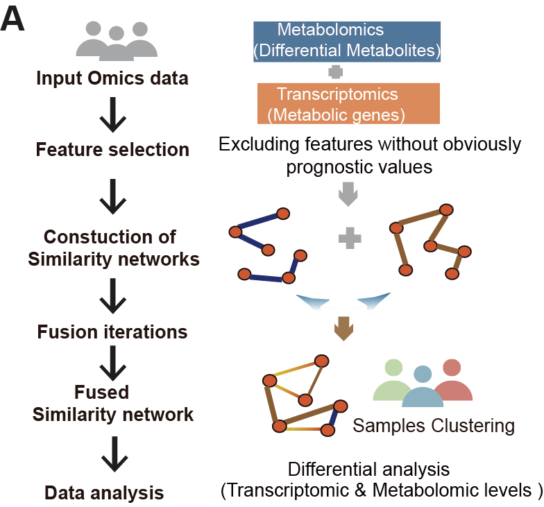
5.2 (B) Discrimination of BCP-ALL Clusters
The discrimination of three clusters (BC1, BC2 and BC3) generated from SNF method.
library(dplyr)
library(MNet)
library(survival)
library(survminer)

#-------------------------------------------------------------------------------
#  Step 1: Load data and set parameters
#-------------------------------------------------------------------------------
dat_filter <- data.table::fread("result/Figure2/1.BMMCvsHC.txt") %>%
  as.data.frame() %>%
  dplyr::arrange(P.Value) %>%
  dplyr::filter(P.Value < 0.5)
dat_filter$P.Value[1:5]

dat_cox <- data.table::fread("result/Figure4/4A_1.cox_metabolite_all_B.txt") %>%
 as.data.frame() %>%
  dplyr::arrange(p.value) %>%
  head(n=120)
dat_cox$p.value[1:5]
dat_filter <- dat_filter %>%
  dplyr::filter(name %in% dat_cox$name_raw)

sample_info <- readxl::read_excel("raw_data/sample_clinical_201_info.xlsx") %>%
  as.data.frame() %>%
  dplyr::filter(!is.na(METc_BM_D0_ID)) %>%
  dplyr::filter(!is.na(RNA_ID)) %>%
  dplyr::filter(Lineage=="B")

dat_cell <- data.table::fread("raw_data/cell_dat_final_reuslt_v0329.txt") %>%
  as.data.frame() %>%
  dplyr::filter(label %in% dat_filter$name) %>%
  tibble::column_to_rownames("label") %>%
  dplyr::select(all_of(sample_info$METc_BM_D0_ID)) %>%
  log1p()

names(dat_cell) <- sample_info$Pid

cox_gene <- data.table::fread("result/Figure4/4A_1.cox_gene_all_B.txt") %>%
  as.data.frame() %>%
  dplyr::arrange(p.value) %>%
  head(n=600)

dat_gene <- readRDS("raw_data/20231113_RNA_ALL_VST_coding.rds") %>%
  as.data.frame() %>%
  dplyr::select(sample_info$RNA_id_raw) %>%
  tibble::rownames_to_column(var="label") %>%
  dplyr::filter(label %in% cox_gene$name_raw) %>%
  tibble::column_to_rownames("label")

names(dat_gene) <- sample_info$Pid

#-------------------------------------------------------------------------------
#  Step 2: SNF of discrimination BCP-ALL clusters
#-------------------------------------------------------------------------------
library(SNFtool)
metabolite_norm = standardNormalization(t(dat_cell))
metgene_norm = standardNormalization(t(dat_gene))

dim(metabolite_norm)
dim(metgene_norm)

write.table(metabolite_norm,"result/Figure4/4B_metabolite_norm_B.txt",quote=F,sep="\t")
write.table(metgene_norm,"result/Figure4/4B_metgene_norm_B.txt",quote=F,sep="\t")

Dist1 = (SNFtool::dist2(as.matrix(metabolite_norm),as.matrix(metabolite_norm)))^(1/2)
Dist2 = (SNFtool::dist2(as.matrix(metgene_norm),as.matrix(metgene_norm)))^(1/2)
W1 = affinityMatrix(Dist1, 10, 0.5)
W2 = affinityMatrix(Dist2, 10, 0.5)
W = SNF(list(W1,W2), 10, 10)

Clusters = spectralClustering(W,K=3)
M_label=cbind(Clusters,sample_info) %>%
  dplyr::mutate(Clusters=ifelse(Clusters==1,"BC3",
                         ifelse(Clusters==2,"BC2",
                         ifelse(Clusters==3,"BC1",Clusters))))

write.table(M_label,paste0("result/Figure4/4B_cluster_B.txt"),quote=F,row.names = F,sep="\t")

library(ComplexHeatmap)
l <- M_label %>%
  dplyr::arrange(Clusters)

W_2 <- W %>%
  as.data.frame() %>%
  dplyr::select(l$Pid) %>%
  tibble::rownames_to_column(var="sample") %>%
  dplyr::arrange(match(sample,l$Pid)) %>%
  tibble::column_to_rownames("sample")
W_2[W_2==0.5] <- 0

col_fun = circlize::colorRamp2(c( 0, 0.03), c( "white","#F48326"))

p_metabolite <- Heatmap(W_2,height=unit(10,"cm"),name="Sample Data",
                        cluster_rows = F,cluster_columns = F,
                        col = col_fun,
                        show_column_names = F,show_row_names = F,
                        row_names_gp = gpar(fontsize = 3),
                        column_names_gp = gpar(fontsize = 3))

pdf("result/Figure4/4B_SNF_discrimination_complexheatmap_B.pdf",width=5,height = 5)
p_metabolite
dev.off()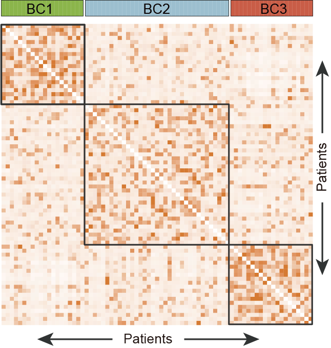
5.3 (C) OS in 75 BCP-ALL patients
The association of the three metabolic clusters with clinical OS in 75 BCP-ALL patients.
library(dplyr)
library(MNet)
library(survival)
library(survminer)

#-------------------------------------------------------------------------------
#  Step 1: Load data
#-------------------------------------------------------------------------------

##### new survival #####
survival_new <- readxl::read_excel("raw_data/Meta_Files.xlsx",skip=1) %>%
  as.data.frame() %>%
  dplyr::select(PID,OS_stat,`OS (days)`) %>%
  dplyr::rename("OS"="OS (days)")

clinical_survival <- data.table::fread(paste0("result/Figure4/4B_cluster_B.txt")) %>%
  as.data.frame() %>%
  dplyr::select(-OS_stat,-OS,-EFS_stat,-EFS,-RFS_stat,-RFS) %>%
  left_join(survival_new,by=c("Pid"="PID"))

#-------------------------------------------------------------------------------
#  Step 2: Overall survival analysis
#-------------------------------------------------------------------------------
surv_object <- Surv(time = clinical_survival$OS/30, event = clinical_survival$OS_stat)
fit_cluster <- survfit(surv_object ~ Clusters, data = clinical_survival)

p1 <- survminer::ggsurvplot(fit_cluster, data = clinical_survival,
                            title="OS",
                            palette=c("#9BD53F","#A6CEE3","#EA644C"),
                            tables.theme = theme_void(),risk.table = TRUE,
                            risk.table.fontsize=6,
                            break.time.by = 12,
                            risk.table.y.text = FALSE,
                            tables.height = 0.15,risk.table.col = "black",
                            #pval = TRUE,pval.method = F,
                            #pval.coord=c(0.5,0.1),pval.size=6,
                            font.tickslab=c(14,"plain","black"),
                            xlab="Time (Months) ",ylab="OS Survival")

pdf(paste0("result/Figure4/4C_OS_B.pdf"),onefile=FALSE)
p1
dev.off()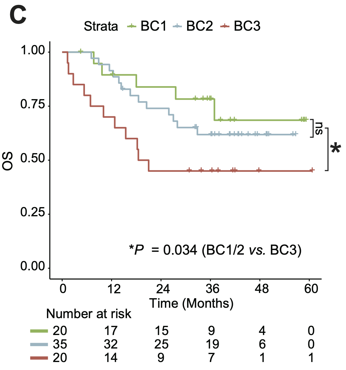
5.4 (D) Multivariate Cox Analysis
The multivariate Cox analysis reveals that the metabolic cluster bore an independent prognostic value for OS and EFS, respectively. The WBC was stratified by 30×109/L. In the genetic-based risk stratification, BCR::ABL1, ETV6::RUNX1, DUX4::IGH and TCF3::PBX1 were categorized into standard risk subgroup, otherwise were into poor risk subgroup.
library(dplyr)
library(openxlsx)
library(survival)
library(survminer)

#-------------------------------------------------------------------------------
#  Step 1: Load data and set parameters
#-------------------------------------------------------------------------------
tt <- readxl::read_excel("raw_data/Sample_RNA_190_fusion_mutation_v1130.xlsx") %>%
  as.data.frame() %>%
  dplyr::select(mutation,fusion,RNA_id,Prediction_Check)

M_label <- data.table::fread("result/Figure4/4B_cluster_B.txt") %>%
  as.data.frame() %>%
  dplyr::mutate(Clusters=ifelse(Clusters %in% c("BC1","BC2"),"BC1+BC2",Clusters)) %>%
  dplyr::mutate(Clusters=as.factor(Clusters)) %>%
  dplyr::select(Clusters,Pid)

##### new survival #####
clinical_survival <- readxl::read_excel("raw_data/Meta_Files.xlsx",skip=1) %>%
  as.data.frame() %>%
  dplyr::rename("OS"="OS (days)","EFS"="EFS (days)","RFS"="RFS (days)","ifHSCT"="HSCT_stat",
         "WBC"="WBC (10⁹/L)","Age"="Age (yrs)","Pid"="PID","RNA_id_raw"="RNA_ID_raw") %>%
  dplyr::select(Pid,RNA_id_raw,Age,Sex,WBC,ifHSCT,OS,OS_stat,EFS,EFS_stat,RFS,RFS_stat,D28_status) %>%
  dplyr::mutate(WBC_type= ifelse(WBC>30, "high",
                                 ifelse(WBC<=30,"low",NA))) %>%
  dplyr::mutate(ifHSCT=as.factor(ifHSCT)) %>%
  dplyr::inner_join(M_label,by="Pid") %>%
  dplyr::left_join(tt,by=c("RNA_id_raw"="RNA_id")) %>%
  dplyr::mutate(NCCN=ifelse(fusion %in% c("ETV6-RUNX1","DUX4-IGH","TCF3-PBX1"),"Standard risk",
                            ifelse(fusion %in% c("KMT2A-AFF1","EP300-ZNF384","SMARCA2-ZNF384"),"Poor risk",
                                   ifelse(Prediction_Check=="Ph-like","Poor risk",
                                          ifelse(Prediction_Check %in% c("BCL2/MYC","PAX5alt","High hyperdoploid", "Low hypodiploid","IDH","TWIST2-high"),"Poor risk","Standard risk"))))) %>%
  dplyr::mutate(NCCN=factor(NCCN,levels=c("Standard risk","Poor risk"))) %>%
  dplyr::mutate(Sex=factor(Sex,levels=c("M","F"))) %>%
  dplyr::mutate(Age=ifelse(Age>40,"old","young")) %>%
  dplyr::mutate(Age=factor(Age,levels=c("young","old")))

var.names <- c("Clusters","WBC_type","Age","NCCN","D28_status","ifHSCT")

#-------------------------------------------------------------------------------
#  Step 2: Event-free survival (EFS)
#-------------------------------------------------------------------------------
f_efs <- as.formula(paste('Surv(EFS, EFS_stat)~',paste(var.names,collapse = "+")))
fit.final <- coxph(f_efs,data=clinical_survival)
p_efs <- ggforest(fit.final,main="EFS Hzard Ratio",
                  cpositions=c(0.02,0.22,0.4),
                  fontsize=0.8,refLabel="reference",
                  noDigits=2,data=clinical_survival)

#-------------------------------------------------------------------------------
#  Step 3: Overall survival(OS)
#-------------------------------------------------------------------------------
f_os <- as.formula(paste('Surv(OS, OS_stat)~',paste(var.names,collapse = "+")))
fit.os <- coxph(f_os,data=clinical_survival)
p_os <- ggforest(fit.os,main="OS Hzard Ratio",
                 cpositions=c(0.02,0.22,0.4),
                 fontsize=0.8,refLabel="reference",
                 noDigits=2,data=clinical_survival)

ggsave(p_efs,filename = "result/Figure4/4D_HR_EFS_B_NCCN_1plus2vs3.pdf",width=9,height=4.5)
ggsave(p_os,filename = "result/Figure4/4D_HR_OS_B_NCCN_1plus2vs3.pdf",width=9,height=4.5)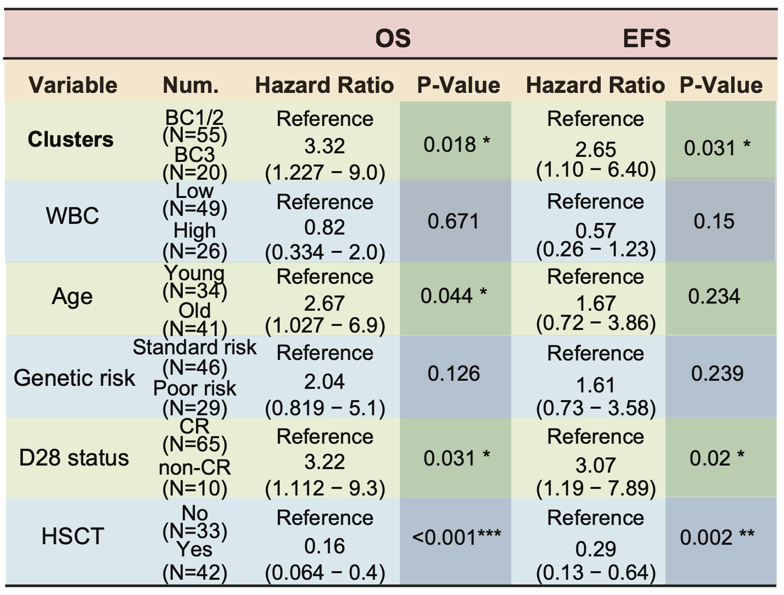
5.5 (E) Subnetwork between BC3 and BC1/2
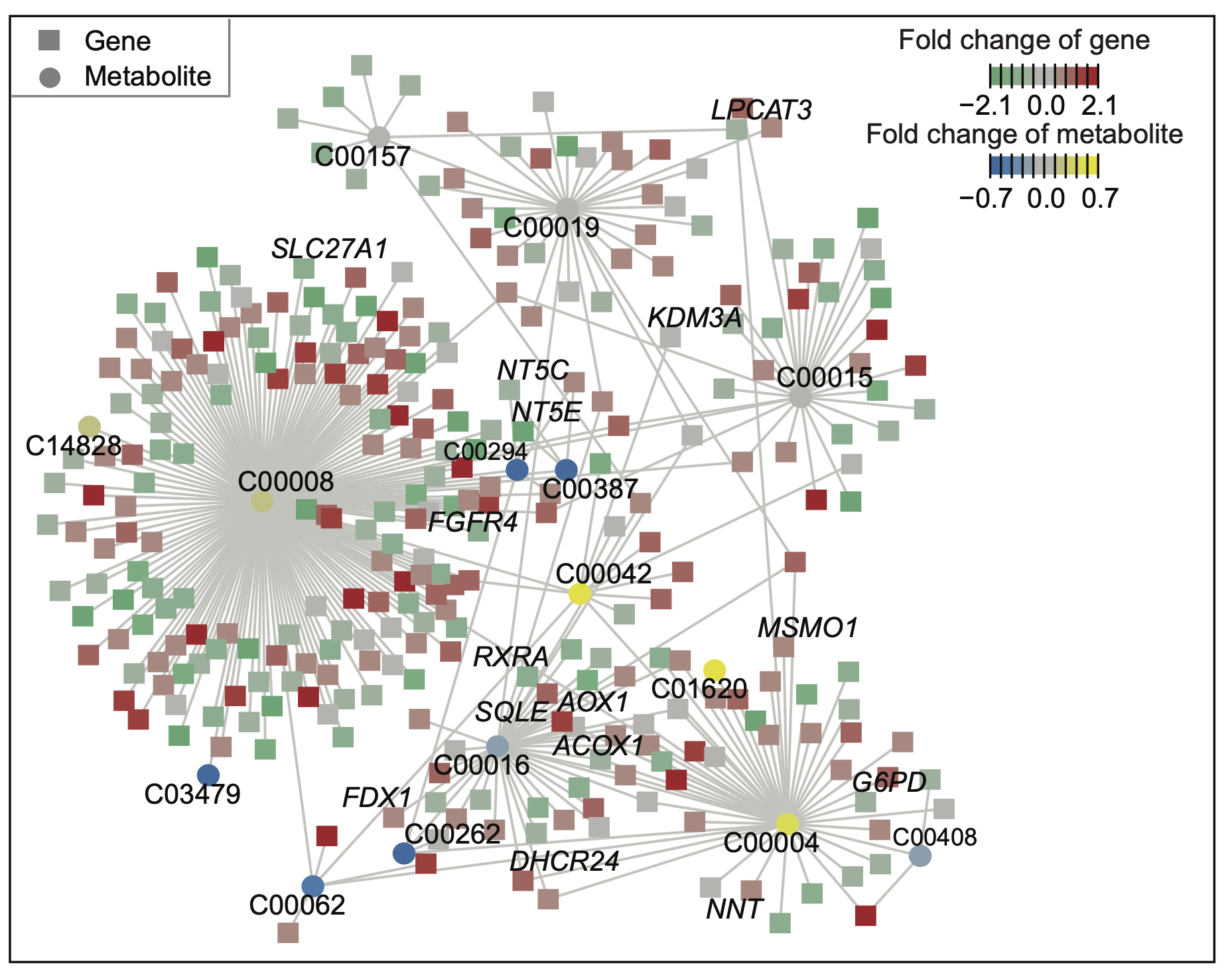
A core metabolism-based subnetwork that best explains the difference between BC3 and BC1/2. In this network, each circular node represents a metabolite, labeled with its KEGG ID, and each square node represents a gene. Node colors indicate logFC values: red and green signify different gene expression levels, while yellow and blue signify varying metabolite levels. The highlighted labels correspond to pathways in the cholesterol metabolism and nicotinate and nicotinamide metabolism.
library(dplyr)
library(ggplot2)
library(igraph)
library(MNet)
library(graphics)
library(cowplot)

rm(list = ls())

#-------------------------------------------------------------------------------
#  Step 1: Read data and set parameters
#-------------------------------------------------------------------------------

gene1 <- readxl::read_excel("raw_data/Chol_Transport_Deg_Ester.xlsx") %>%
  as.data.frame()

name_gene <- data.table::fread("result/Figure4/4A_1.cox_gene_all_B.txt") %>%
  as.data.frame()

diff_gene <- data.table::fread("result/Figure4/S5H_gene_B.txt") %>%
  as.data.frame() %>%
  filter(name %in% name_gene$name_raw)

kid <- openxlsx::read.xlsx("raw_data/cell_metabolite_info_all_v1109.xlsx") %>%
  as.data.frame() %>%
  dplyr::select(refmet_name,KEGG) %>%
  mutate(KEGG=ifelse(KEGG=="None",refmet_name,KEGG))

diff_meta <- data.table::fread("result/Figure4/S5H_metabolite_B.txt") %>%
  as.data.frame() %>%
  inner_join(kid,by=c("name"="refmet_name")) %>%
  dplyr::select(-name) %>%
  dplyr::rename("name"="KEGG") %>%
  arrange(P.Value) %>%
  distinct(name,.keep_all = T)

names(diff_meta)[4]  <- "p_value"

names(diff_gene)[4] <- "p_value"

dd <- data.table::fread("raw_data/subnetwork_important_edge-300_B.txt") %>%
  as.data.frame()

set.seed(1)
g <- graph_from_data_frame(dd)
layout <- layout_with_dh(g,set.seed(1))
row.names(layout) <- names(V(g))
colnames(layout) <- c("pos.x","pos.y")

kk <- PathwayExtendData %>%
  filter(kegg_pathwayname=="Nicotinate and nicotinamide metabolism")

node.data <- as.data.frame(layout) %>%
  tibble::rownames_to_column(var="label") %>%
  left_join(diff_gene,by=c("label"="name")) %>%
  left_join(diff_meta,by=c("label"="name")) %>%
  dplyr::select(label,pos.x,pos.y,logFC.x,logFC.y) %>%
  mutate(logFC=ifelse(is.na(logFC.x),logFC.y,logFC.x)) %>%
  mutate(type=ifelse(is.na(logFC.x),"metabolite","gene")) %>%
  dplyr::select(-logFC.x,-logFC.y) %>%
  mutate(label1=ifelse(label %in% gene1$`Gene Name` |label %in% kk$name| type=="metabolite",label,NA))

ab <- node.data %>%
  filter(!is.na(label1)) %>%
  left_join(gene1,by=c("label1"="Gene Name"))
write.table(ab,"result/Figure4/4E_node-filter.txt",quote=F,row.names = F,sep="\t")

edge.data <- dd %>%
  dplyr::rename("fromNode"="X1",
         "toNode"="X2") %>%
  dplyr::select(fromNode,toNode) %>%
  dplyr::left_join(node.data,by=c("fromNode"="label")) %>%
  dplyr::rename("from.x"="pos.x","from.y"="pos.y") %>%
  dplyr::left_join(node.data,by=c("toNode"="label")) %>%
  dplyr::rename("to.x"="pos.x","to.y"="pos.y")

#-------------------------------------------------------------------------------
#  Step 2: Core metabolism-based subnetwork
#-------------------------------------------------------------------------------
## node.color
source("raw_data/node.color.R")
source("raw_data/col.key.R")
source("raw_data/colorpanel2.R")

node_meta <- node.data %>%
  filter(type=="metabolite") %>%
  mutate(logFC=round(logFC,2)) %>%
  mutate(logFC=ifelse(logFC < -0.58, -0.58, logFC))
meta_limits=as.numeric(sprintf("%.1f", max(max(node_meta$logFC),abs(min(node_meta$logFC)))))+0.1
meta_color <- node.color(limit=meta_limits,node_meta$logFC,low="#007DDB", mid="gray", high="yellow")
node_meta$color <- meta_color

node_gene <- node.data %>%
  filter(type=="gene") %>%
  mutate(logFC=round(logFC,2)) %>%
  mutate(logFC=ifelse(logFC < -2, -2, logFC)) %>%
  mutate(logFC=ifelse(logFC > 2, 2, logFC))
gene_limits=as.numeric(sprintf("%.1f", max(max(node_gene$logFC),abs(min(node_gene$logFC)))))+0.1
gene_color <- node.color(limit=gene_limits,node_gene$logFC,low="#4FBD81",mid="gray",high="#D01910")
node_gene$color <- gene_color

node.data1 <- rbind(node_meta,node_gene)

aa=node.data1$color
names(aa)=node.data1$color

gg <- ggplot()
gg <- gg + geom_segment(mapping = aes(x = from.x, y = from.y, xend = to.x, yend = to.y),
                        color = "#CCCCCC", size = 0.5, data = edge.data)
gg <- gg + geom_point(mapping = aes(x = pos.x, y = pos.y,color=color,shape=type),
                      size = 4, data = node.data1)
gg <- gg + scale_size(range = c(0, 6) * 2)
gg <- gg + theme_void()+theme(legend.position="none")
gg <- gg + labs(x = "", y = "")
gg <- gg + ggrepel::geom_text_repel(mapping=aes(x = pos.x, y = pos.y,label=label1),data=node.data1)
gg <- gg + scale_colour_manual(values = aa)+scale_shape_manual(values=c("gene"="square","metabolite"="circle"))

p <- plot.new()
off.sets=col.key(limit=gene_limits,bins=10,cex=0.5,graph.size = c(1,1),off.sets=c(x=0,y=0),
                 low="#4FBD81",mid="gray",high="#D01910")
off.sets=col.key(limit=meta_limits,bins=10,cex=0.5,low="#007DDB", mid="gray", high="yellow",
                   off.sets=c(x=0,y=0),graph.size = c(1,0.9))
p <- recordPlot()
dev.off()

p1 <- ggdraw()+
  draw_plot(p,0.5,0.5,0.5,0.55)+
  draw_plot(gg,0,0,1,1)

ggsave("result/Figure4/4E_node-300-all-B.pdf",p1,width=6,height = 6)

if (0) {
  png("result/Figure4/4E_node-300-aa.png",width=5,height = 5,units = 'in', res = 200)
  grid::grid.draw(p1)
  dev.off()
}
5.6 (F) Discrimination of T-ALL Clusters
The discrimination of two T-ALL clusters (TC1 and TC2) based on SNF method.
library(dplyr)
library(MNet)
library(survival)
library(survminer)

#-------------------------------------------------------------------------------
#  Step 1: Load data and set parameters
#-------------------------------------------------------------------------------
dat_filter <- data.table::fread("result/Figure2/1.BMMCvsHC.txt") %>%
  as.data.frame() %>%
  dplyr::arrange(P.Value) %>%
  dplyr::filter(P.Value < 0.5)
dat_filter$P.Value[1:5]

dat_cox <- data.table::fread("result/Figure4/4A_1.cox_metabolite_all_T.txt") %>%
 as.data.frame() %>%
  dplyr::arrange(p.value) %>%
  head(n=120)
dat_cox$p.value[1:5]
dat_filter <- dat_filter %>%
  dplyr::filter(name %in% dat_cox$name_raw)

sample_info <- readxl::read_excel("raw_data/sample_clinical_201_info.xlsx") %>%
  as.data.frame() %>%
  dplyr::filter(!is.na(METc_BM_D0_ID)) %>%
  dplyr::filter(!is.na(RNA_ID)) %>%
  dplyr::filter(Lineage=="T")

dat_cell <- data.table::fread("raw_data/cell_dat_final_reuslt_v0329.txt") %>%
  as.data.frame() %>%
  dplyr::filter(label %in% dat_filter$name) %>%
  tibble::column_to_rownames("label") %>%
  dplyr::select(all_of(sample_info$METc_BM_D0_ID)) %>%
  log1p()

names(dat_cell) <- sample_info$Pid

cox_gene <- data.table::fread("result/Figure4/4A_1.cox_gene_all_T.txt") %>%
  as.data.frame() %>%
  dplyr::arrange(p.value) %>%
  head(n=600)

dat_gene <- readRDS("raw_data/20231113_RNA_ALL_VST_coding.rds") %>%
  as.data.frame() %>%
  dplyr::select(sample_info$RNA_id_raw) %>%
  tibble::rownames_to_column(var="label") %>%
  dplyr::filter(label %in% cox_gene$name_raw) %>%
  tibble::column_to_rownames("label")

names(dat_gene) <- sample_info$Pid

#-------------------------------------------------------------------------------
#  Step 2: SNF of discrimination T-ALL clusters
#-------------------------------------------------------------------------------
library(SNFtool)
metabolite_norm = standardNormalization(t(dat_cell))
metgene_norm = standardNormalization(t(dat_gene))

dim(metabolite_norm)
dim(metgene_norm)

write.table(metabolite_norm,"result/Figure4/4F_metabolite_norm_T.txt",quote=F,sep="\t")
write.table(metgene_norm,"result/Figure4/4F_metgene_norm_T.txt",quote=F,sep="\t")

Dist1 = (SNFtool::dist2(as.matrix(metabolite_norm),as.matrix(metabolite_norm)))^(1/2)
Dist2 = (SNFtool::dist2(as.matrix(metgene_norm),as.matrix(metgene_norm)))^(1/2)
W1 = affinityMatrix(Dist1, 10, 0.5)
W2 = affinityMatrix(Dist2, 10, 0.5)
W = SNF(list(W1,W2), 10, 10)

Clusters = spectralClustering(W,K=2)
M_label=cbind(Clusters,sample_info) %>%
  dplyr::mutate(Clusters=ifelse(Clusters==1,"TC2",
                                ifelse(Clusters==2,"TC1",Clusters)))
write.table(M_label,paste0("result/Figure4/4F_cluster_T.txt"),quote=F,row.names = F,sep="\t")

l <- M_label %>%
  dplyr::arrange(Clusters)

W_2 <- W %>%
  as.data.frame() %>%
  dplyr::select(l$Pid) %>%
  tibble::rownames_to_column(var="sample") %>%
  dplyr::arrange(match(sample,l$Pid)) %>%
  tibble::column_to_rownames("sample")
W_2[W_2==0.5] <- 0

col_fun = circlize::colorRamp2(c( 0, 0.03), c( "white","#F48326"))

library(ComplexHeatmap)
p_metabolite <- Heatmap(W_2,height=unit(10,"cm"),name="Sample Data",
                        cluster_rows = F,cluster_columns = F,
                        col = col_fun,
                        #top_annotation =top_annotation,
                        show_column_names = F,show_row_names = F,
                        row_names_gp = gpar(fontsize = 3),column_names_gp = gpar(fontsize = 3))

pdf("result/Figure4/4F_SNF_discrimination_complexheatmap_T.pdf",width=5,height = 5)
p_metabolite
dev.off()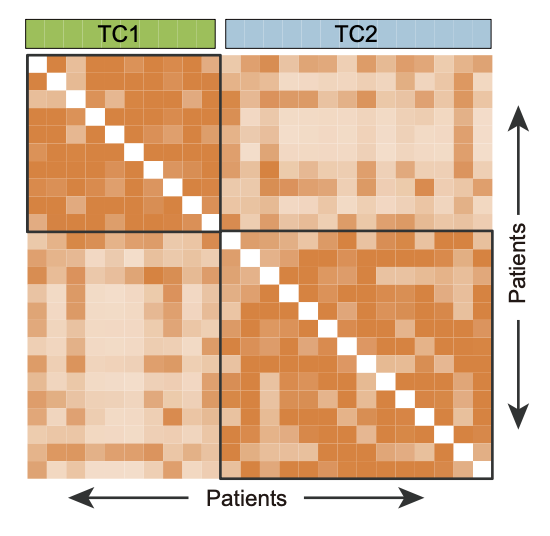
5.7 (G) OS of TC1/2
The association of the two metabolic clusters with clinical OS outcomes in 24 T-ALL patients. The result suggested TC1 was of significantly poorer prognosis than TC2.
library(dplyr)
library(MNet)
library(survival)
library(survminer)

#------------------------------------------------------------------------------
#  OS of TC1/2
#------------------------------------------------------------------------------
##### new survival #####
survival_new <- readxl::read_excel("raw_data/Meta_Files.xlsx",skip=1) %>%
  as.data.frame() %>%
  dplyr::select(PID,OS_stat,`OS (days)`) %>%
  dplyr::rename("OS"="OS (days)")

clinical_survival <- data.table::fread(paste0("result/Figure4/4F_cluster_T.txt")) %>%
  as.data.frame() %>%
  dplyr::select(-OS_stat,-OS,-EFS_stat,-EFS,-RFS_stat,-RFS) %>%
  left_join(survival_new,by=c("Pid"="PID"))

surv_object <- Surv(time = clinical_survival$OS/30, event = clinical_survival$OS_stat)
fit_cluster <- survfit(surv_object ~ Clusters, data = clinical_survival)
p1 <- survminer::ggsurvplot(fit_cluster, data = clinical_survival,
                            title="OS",
                            palette=c("#9BD53F","#A6CEE3"),
                            tables.theme = theme_void(),risk.table = TRUE,
                            risk.table.fontsize=6,
                            break.time.by = 12,
                            risk.table.y.text = FALSE,
                            tables.height = 0.15,risk.table.col = "black",
                            pval = TRUE,
                            pval.method = F,pval.coord=c(0.5,0.1),pval.size=6,
                            font.tickslab=c(14,"plain","black"),
                            xlab="Time (Months) ",ylab="OS Survival")

pdf(paste0("result/Figure4/4G_OS_T.pdf"),onefile=FALSE)
p1
dev.off()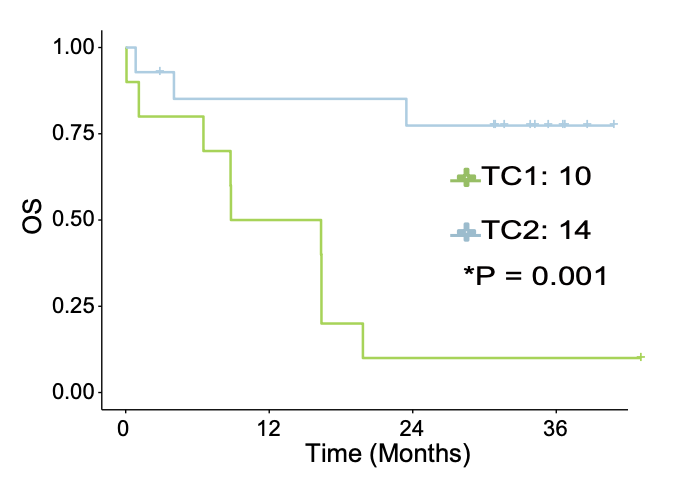
5.8 (H) Subnetwork between TC2 and TC1
A core metabolism-based subnetwork that best explains the difference between TC2 and TC1. The highlighted labels correspond to pathways in the TCA and OXPHOS. PC refers to a group of phosphatidylcholines without specific KEGG IDs.
library(dplyr)
library(ggplot2)
library(igraph)
library(MNet)
library(graphics)
library(cowplot)

#-------------------------------------------------------------------------------
#  Step 1: Read data and set parameters
#-------------------------------------------------------------------------------

rm(list = ls())
name_gene <- data.table::fread("result/Figure4/4A_1.cox_gene_all_T.txt") %>%
  as.data.frame()

diff_gene <- data.table::fread("result/Figure4/S6J_gene_T.txt") %>%
  as.data.frame() %>%
  filter(name %in% name_gene$name_raw)

kid <- openxlsx::read.xlsx("raw_data/cell_metabolite_info_all_v1109.xlsx") %>%
  as.data.frame() %>%
  dplyr::select(refmet_name,KEGG) %>%
  mutate(KEGG=ifelse(KEGG=="None",refmet_name,KEGG))

diff_meta <- data.table::fread("result/Figure4/S6J_metabolite_T.txt") %>%
  as.data.frame() %>%
  inner_join(kid,by=c("name"="refmet_name")) %>%
  dplyr::select(-name) %>%
  dplyr::rename("name"="KEGG") %>%
  arrange(P.Value) %>%
  distinct(name,.keep_all = T)

names(diff_meta)[4]  <- "p_value"

names(diff_gene)[4] <- "p_value"

dd <- data.table::fread("raw_data/subnetwork_important_edge-300_T.txt") %>%
  as.data.frame()

set.seed(2)
g <- graph_from_data_frame(dd)
layout <- layout_with_dh(g,set.seed(1))
row.names(layout) <- names(V(g))
colnames(layout) <- c("pos.x","pos.y")

kk <- PathwayExtendData %>%
  filter(kegg_pathwayname %in% c("Citrate cycle (TCA cycle)","Oxidative phosphorylation"))

node.data <- as.data.frame(layout) %>%
  tibble::rownames_to_column(var="label") %>%
  left_join(diff_gene,by=c("label"="name")) %>%
  left_join(diff_meta,by=c("label"="name")) %>%
  dplyr::select(label,pos.x,pos.y,logFC.x,logFC.y) %>%
  mutate(logFC=ifelse(is.na(logFC.x),logFC.y,logFC.x)) %>%
  mutate(type=ifelse(is.na(logFC.x),"metabolite","gene")) %>%
  dplyr::select(-logFC.x,-logFC.y) %>%
  mutate(label1=ifelse(label %in% kk$name,label,NA))

edge.data <- dd %>%
  dplyr::rename("fromNode"="X1",
         "toNode"="X2") %>%
  dplyr::select(fromNode,toNode) %>%
  dplyr::left_join(node.data,by=c("fromNode"="label")) %>%
  dplyr::rename("from.x"="pos.x","from.y"="pos.y") %>%
  dplyr::left_join(node.data,by=c("toNode"="label")) %>%
  dplyr::rename("to.x"="pos.x","to.y"="pos.y")

## node.color
source("raw_data/node.color.R")
source("raw_data/col.key.R")
source("raw_data/colorpanel2.R")

node_meta <- node.data %>%
  filter(type=="metabolite") %>%
  mutate(logFC=round(logFC,2)) %>%
  mutate(logFC=ifelse(logFC < -0.58, -0.58, logFC))
meta_limits=as.numeric(sprintf("%.1f", max(max(node_meta$logFC),abs(min(node_meta$logFC)))))+0.1
meta_color <- node.color(limit=meta_limits,node_meta$logFC,low="#007DDB", mid="gray", high="yellow")
node_meta$color <- meta_color

node_gene <- node.data %>%
  filter(type=="gene") %>%
  mutate(logFC=round(logFC,2)) %>%
  mutate(logFC=ifelse(logFC < -2, -2, logFC)) %>%
  mutate(logFC=ifelse(logFC > 2, 2, logFC))
gene_limits=as.numeric(sprintf("%.1f", max(max(node_gene$logFC),abs(min(node_gene$logFC)))))+0.1
gene_color <- node.color(limit=gene_limits,node_gene$logFC,low="#4FBD81",mid="gray",high="#D01910")
node_gene$color <- gene_color

node.data1 <- rbind(node_meta,node_gene)

aa=node.data1$color
names(aa)=node.data1$color

gg <- ggplot()
gg <- gg + geom_segment(mapping = aes(x = from.x, y = from.y, xend = to.x, yend = to.y),
                        color = "#CCCCCC", size = 0.5, data = edge.data)
gg <- gg + geom_point(mapping = aes(x = pos.x, y = pos.y,color=color,shape=type),
                      size = 4, data = node.data1)
gg <- gg + scale_size(range = c(0, 6) * 2)
gg <- gg + theme_void()+theme(legend.position="none")
gg <- gg + labs(x = "", y = "")
gg <- gg + ggrepel::geom_text_repel(mapping=aes(x = pos.x, y = pos.y,label=label1),data=node.data1)
gg <- gg + scale_colour_manual(values = aa)+scale_shape_manual(values=c("gene"="square","metabolite"="circle"))

pdf("result/Figure4/4H_node-200-1_T.pdf")
p <- plot.new()
off.sets=col.key(limit=gene_limits,bins=10,cex=0.5,graph.size = c(1,1),off.sets=c(x=0,y=0),
                 low="#4FBD81",mid="gray",high="#D01910")
off.sets=col.key(limit=meta_limits,bins=10,cex=0.5,low="#007DDB", mid="gray", high="yellow",
                   off.sets=c(x=0,y=0),graph.size = c(1,0.9))
p <- recordPlot()
dev.off()

if (0) {
p1 <- ggdraw()+
  draw_plot(p,0.5,0.5,0.5,0.55)+
  draw_plot(gg,0,0,1,1)
ggsave("result/Figure4/4H_node-300-all.pdf",p1,width=6,height = 6)
}

ggsave("result/Figure4/4H_node-300-2_T.pdf",gg,width=6,height = 6)


if (0) {
  png("result/Figure4/4H_node-300-aa.png",width=5,height = 5,units = 'in', res = 200)
  grid::grid.draw(p1)
  dev.off()
}
5.9 (S5 A) Clusters of BCP-ALL
The relative abundance of input metabolites and expression level of metabolic genes in the three metabolic clusters in BCP-ALL: BC1 (N=20), BC2 (N=35), and BC3 (N=20). Each column represents a sample and each row represents a metabolite (upper panel) or gene included (lower panel).
#------------------------------------------------------------------------------
#  Step 1: Heatmap
#------------------------------------------------------------------------------
library(dplyr)
library(ComplexHeatmap)

sample_info <- data.table::fread("result/Figure4/4B_cluster_B.txt") %>%
  as.data.frame()

metabolite_norm = data.table::fread("result/Figure4/4B_metabolite_norm_B.txt") %>%
  as.data.frame() %>%
  tibble::column_to_rownames("V1")

metgene_norm <- data.table::fread("result/Figure4/4B_metgene_norm_B.txt") %>%
  as.data.frame() %>%
  tibble::column_to_rownames("V1")

top_annotation = HeatmapAnnotation(Subtype=sample_info$Clusters,
  col=list(Subtype=c("BC1"="#9BD53F","BC2"="#A6CEE3","BC3"="#EA644C")),
  show_annotation_name = c(T,T),
  border = c(T,T) ,
  simple_anno_size = unit(4, "mm"),gap = unit(1, "mm"))

col_fun = circlize::colorRamp2(c(-1, 0, 1), c("#00599F", "white", "#D01910"))

p_metabolite <- Heatmap(t(metabolite_norm),height=unit(10,"cm"),name="Metabolite Data",
                        cluster_row_slices = F,clustering_method_rows = "ward.D",
                        clustering_method_columns = "ward.D2",
                        column_split = sample_info$Clusters,
                        col = col_fun,
                        top_annotation =top_annotation,
                        show_column_names = F,show_row_names = F,
                        row_names_gp = gpar(fontsize = 3),
                        column_names_gp = gpar(fontsize = 3))

col_fun = circlize::colorRamp2(c(-1, 0, 1), c("#00599F", "white", "#FF7F00"))

p_gene <- Heatmap(t(metgene_norm),height=unit(10,"cm"),name="Gene Data",
                  cluster_row_slices = F,clustering_method_rows = "ward.D",
                  clustering_method_columns = "ward.D2",
                  column_split = sample_info$Clusters,
                  col = col_fun,
                  show_column_names = F,show_row_names = F,
                  row_names_gp = gpar(fontsize = 3),
                  column_names_gp = gpar(fontsize = 3))

pdf(paste0("result/Figure4/S5A_heatmap_B.pdf"),width=8,height = 10)
p_metabolite %v% p_gene
dev.off()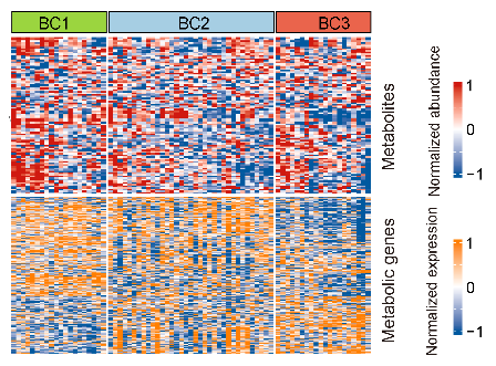
5.10 (S5 G) Waterfall plot of BC1/2/3
The associations of metabolic clusters with clinical variables and genetic alterations, including major mutations and fusions in BCP-ALL. Note: Among all fusions, only BCR::ABL1 and TCF3::PBX1 were significantly enriched in BC1/2 and BC3, respectively. P-value was calculated by Pearson’s chi-square test or Fisher’s exact test.
library(dplyr)
library(ComplexHeatmap)

#-------------------------------------------------------------------------------
#  Step 1: Load data and set parameters
#-------------------------------------------------------------------------------

clinical_survival <- readxl::read_excel("raw_data/Meta_Files.xlsx",skip=1) %>%
  as.data.frame() %>%
  dplyr::rename("OS"="OS (days)","EFS"="EFS (days)","RFS"="RFS (days)","ifHSCT"="HSCT_stat",
         "WBC"="WBC (10⁹/L)","Age"="Age (yrs)","Pid"="PID","RNA_id_raw"="RNA_ID_raw") %>%
  dplyr::select(Pid,RNA_id_raw,Age,Sex,WBC,ifHSCT,OS_stat,D28_status) %>%
  #dplyr::mutate(Age=ifelse(Age < 40,"< 40",">= 40")) %>%
  dplyr::mutate(WBC_type= ifelse(WBC>30, "> 30",
                                 ifelse(WBC<=30,"<= 30",NA))) %>%
  dplyr::mutate(Outcome=ifelse(OS_stat==1,"Dead",
                               ifelse(OS_stat==0,"Alive",OS_stat))) %>%
  dplyr::mutate(ifHSCT=ifelse(ifHSCT==0,"no",
                              ifelse(ifHSCT==1,"yes",ifHSCT)))

sample_info_raw <- data.table::fread("raw_data/1.cluster_B.txt") %>%
  as.data.frame() %>%
  dplyr::select(bianhao,Clusters)

sample_info <- data.table::fread("result/Figure4/4B_cluster_B.txt") %>%
  as.data.frame() %>%
  dplyr::select(Clusters,Pid) %>%
  dplyr::mutate(bianhao=gsub("RJ-","A",Pid)) %>%
  dplyr::arrange(match(bianhao,sample_info_raw$bianhao)) %>%
  dplyr::left_join(clinical_survival,by="Pid") %>%
  dplyr::rename("RNA_id"="RNA_id_raw")

#-------------------------------------------------------------------------------
#  Step 2: Mutations
#-------------------------------------------------------------------------------
q12 <- c("#1F78B4","#E31A1C","black")
names(q12) <- unique(sample_info$Clusters)

top_annotation = HeatmapAnnotation(
  Subtype=sample_info$Clusters,
  #Age=sample_info$Age,
  ifHSCT=sample_info$ifHSCT,
  WBC=sample_info$WBC_type,
  Outcome=sample_info$Outcome,
  col=list(Subtype=c("BC1"="#9BD53F","BC2"="#A6CEE3","BC3"="#EA644C"),
           Age=c("< 40"="#B2DF8A",">= 40"="gray"),
           ifHSCT=c("yes"="#CAB2D6","no"="gray"),
           WBC=c("> 30"="#FDBF6F","<= 30"="gray"),
           Outcome=c("Dead"="black","Alive"="gray")),
  show_annotation_name = c(T,T),
  border = c(T,T,T,T,T,T) ,
  simple_anno_size = unit(8, "mm"),gap = unit(1.5, "mm"))

mutation_B <- data.table::fread("raw_data/mutation_B_v1114_all.txt") %>%
  as.data.frame() %>%
  dplyr::select(V2,V17,V19) %>%
  dplyr::rename("ID"="V2","Gene.refGene"="V17","ExonicFunc.refGene"="V19") %>%
  dplyr::select(ID,`Gene.refGene`,`ExonicFunc.refGene`) %>%
  dplyr::mutate(`ExonicFunc.refGene`=
                  ifelse(`ExonicFunc.refGene` %in% c("frameshift deletion","frameshift insertion","frameshift substitution"),"Frameshift",
                         ifelse(`ExonicFunc.refGene` %in% c("nonframeshift deletion","nonframeshift insertion","nonframeshift substitution"),"Nonframeshift",
                                ifelse(`ExonicFunc.refGene` %in% ".","Splice",
                                       ifelse(`ExonicFunc.refGene` %in% "nonsynonymous SNV","Missense",
                                              ifelse(`ExonicFunc.refGene`=="startloss","Startloss",
                                                     ifelse(`ExonicFunc.refGene`=="stopgain","Stopgain",
                                                            ifelse(`ExonicFunc.refGene`=="synonymous SNV","Silent",`ExonicFunc.refGene`)))))))) %>%
  unique() %>%
  dplyr::filter(ID %in% sample_info$RNA_id) %>%
  dplyr::mutate(`Gene.refGene` = ifelse(`Gene.refGene` %in% c("IDH1","IDH2"),"IDH1/2",`Gene.refGene`))

mutation <- rbind(mutation_B)

hit_num <- mutation %>%
  dplyr::group_by(ID,`Gene.refGene`) %>%
  dplyr::summarise(n=n()) %>%
  dplyr::filter(n>1)

mutation <- mutation %>%
  dplyr::left_join(hit_num,by=c("ID","Gene.refGene")) %>%
  dplyr::mutate(`ExonicFunc.refGene`=ifelse(!is.na(n),"Multiple",`ExonicFunc.refGene`)) %>%
  dplyr::select(-n) %>%
  unique() %>%
  dplyr::rename("RNA_id"="ID") %>%
  dplyr::filter(RNA_id %in% sample_info$RNA_id)

mutation_gene_filter <- mutation %>%
  dplyr::select(RNA_id,Gene.refGene) %>%
  unique() %>%
  dplyr::group_by(`Gene.refGene`) %>%
  dplyr::summarise(n=n()) %>%
  dplyr::filter(n>0)
mutation_sort <- rev(names(sort(table(mutation %>% filter(`Gene.refGene` %in% mutation_gene_filter$Gene.refGene) %>% pull(Gene.refGene)))))

mutation <- mutation %>%
  dplyr::filter(`Gene.refGene` %in% mutation_gene_filter$Gene.refGene) %>%
  as.data.frame() %>%
  dplyr::distinct(RNA_id,Gene.refGene,.keep_all = T)

sample_info_filter <- sample_info %>%
  dplyr::select(bianhao,RNA_id)

mutation_dcast <- reshape2::dcast(mutation,RNA_id ~ `Gene.refGene`) %>%
  dplyr::right_join(sample_info_filter,by="RNA_id") %>%
  dplyr::select(-RNA_id) %>%
  tibble::column_to_rownames("bianhao") %>%
  dplyr::select(all_of(mutation_sort))

mutation_dcast[is.na(mutation_dcast)] <- 0
mutation_dcast[mutation_dcast=="Missense"] <- 1
mutation_dcast[mutation_dcast=="Frameshift"] <- 2
mutation_dcast[mutation_dcast=="Nonframeshift"] <- 3
mutation_dcast[mutation_dcast=="Silent"] <- 4
mutation_dcast[mutation_dcast=="Splice"] <- 5
mutation_dcast[mutation_dcast=="Stopgain"] <- 7
mutation_dcast[mutation_dcast=="Multiple"] <- 8

mutation_dcast1 <- mutation_dcast %>%
  dplyr::mutate_if(is.character,as.numeric) %>%
  rowwise() %>%
  dplyr::mutate(Signaling=sum(NRAS,KRAS,FLT3,STAT5B,NF1,MYC)) %>%
  dplyr::mutate(Transcription=sum(PAX5,TP53,RUNX1,IKZF1,ETV6,MGA)) %>%
  dplyr::mutate(Epigenetic=sum(KMT2D,SETD2,NCOR2,EP300,ARID1A,ARID1B,SETD1B,`IDH1/2`)) %>%
  dplyr::mutate(Others=sum(SACS)) %>%
  dplyr::mutate(Signaling=ifelse(Signaling==0,0,9)) %>%
  dplyr::mutate(Transcription=ifelse(Transcription==0,0,9)) %>%
  dplyr::mutate(Epigenetic=ifelse(Epigenetic==0,0,9)) %>%
  dplyr::mutate(Others=ifelse(Others==0,0,9)) %>%
  dplyr::select(NRAS,FLT3,STAT5B,NF1,KRAS,MYC,Signaling,
                PAX5,TP53,RUNX1,IKZF1,ETV6,MGA,Transcription,
                KMT2D,SETD2,NCOR2,EP300,ARID1A,ARID1B,SETD1B,`IDH1/2`,Epigenetic,
                SACS,Others) %>%
  as.data.frame()

rownames(mutation_dcast1) <- rownames(mutation_dcast)
mutation_dcast <- mutation_dcast1

mutation_dcast_temp <- mutation_dcast
mutation_dcast_temp[mutation_dcast_temp!=0] <- 1
num=colSums(mutation_dcast_temp)
names(mutation_dcast) <- paste0(names(mutation_dcast)," (n=",num,")")

d_mutation <- t(mutation_dcast) %>%
  as.data.frame() %>%
  dplyr::select(sample_info$bianhao)

mutation_annotation <- Heatmap(d_mutation,height=unit(12,"cm"),rect_gp = gpar(col = "gray", lwd = 2),
                               col=c("#EEEEEE","#3987CC","#DB3D3D","#663FFB","#FF7F0E","#CC66FF","#8B564C","#339933","blue"),
                               cluster_columns = F,cluster_rows = F,border = TRUE,column_title = NULL,
                               column_split =sample_info$Clusters,
                               show_column_names = TRUE,
                               top_annotation=top_annotation,
                               row_names_gp = gpar(fontsize = 10),column_names_gp=gpar(fontsize=6))

#-------------------------------------------------------------------------------
#  Step 3: Fusions
#-------------------------------------------------------------------------------
fusion_B <- readxl::read_excel("raw_data/fusion_B_v0803.xlsx",skip=1) %>%
  as.data.frame() %>%
  dplyr::filter(RNA_id %in% sample_info$RNA_id) %>%
  dplyr::select(RNA_id,fusion_group) %>%
  dplyr::mutate(fusion_group=ifelse(fusion_group %in% c("PAX5-ETV6","PAX5-CPLX1"),"PAX5 fusion",
                                    fusion_group)) %>%
  dplyr::mutate(fusion_group=ifelse(fusion_group=="BCR-ABL1;IKZF1-IGH","BCR-ABL1",fusion_group)) %>%
  dplyr::left_join(sample_info,by="RNA_id") %>%
  dplyr::filter(fusion_group %in% c("BCL2/MYC","BCR-ABL1","DUX4 rearrangement","ETV6-RUNX1","KMT2A rearrangement","PAX5 fusion","TCF3-PBX1","ZNF384 fusion")) %>%
  dplyr::select(RNA_id,fusion_group) %>%
  dplyr::filter(!is.na(fusion_group))

fusion <- rbind(fusion_B)

clinical_fusion_dcast <- reshape2::dcast(fusion,RNA_id ~ fusion_group) %>%
  dplyr::right_join(sample_info_filter,by="RNA_id") %>%
  tibble::column_to_rownames("bianhao") %>%
  dplyr::select(-RNA_id)

clinical_fusion_dcast[is.na(clinical_fusion_dcast)] <- 0
clinical_fusion_dcast[clinical_fusion_dcast != 0] <- 1

d_fusion <- t(clinical_fusion_dcast) %>%
  as.data.frame() %>%
  dplyr::select(sample_info$bianhao) %>%
  tibble::rownames_to_column(var="fusion") %>%
  dplyr::arrange(match(fusion,c("DUX4 rearrangement","ZNF384 fusion","TCF3-PBX1","KMT2A rearrangement","ETV6-RUNX1","PAX5-ETV6","PAX5 fusion","BCL2/MYC"))) %>%
  tibble::column_to_rownames("fusion")

fusion_annotation <- Heatmap(d_fusion,rect_gp = gpar(col = "gray", lwd = 2),
                             col=c("#EEEEEE","#444444"),
                             height=unit(4,"cm"),border = TRUE,
                             column_split =sample_info$Clusters,
                             cluster_columns = F,cluster_rows = F,
                             column_title = NULL,
                             row_names_gp = gpar(fontsize = 10),
                             column_names_gp=gpar(fontsize=6))

pdf(paste0("result/Figure4/S5G_oncoplot_B.pdf"),width=10,height = 10)
mutation_annotation %v% fusion_annotation
dev.off()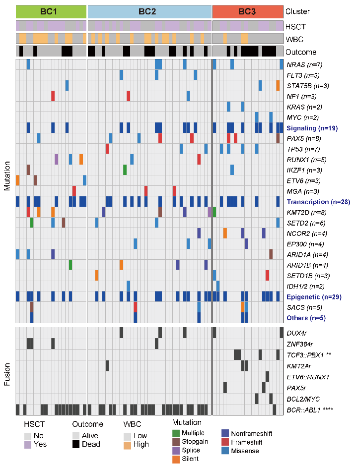
5.11 (S5 H) DA score of BC3 cluster
The DA score reveals that most of the disturbed metabolism pathways are significantly enriched in the BC3 cluster.
library(ggplot2)
library(MNet)
library(dplyr)

#------------------------------------------------------------------------------
#  Stpe 1: mlimma of BCP-ALL clusters
#------------------------------------------------------------------------------
cluster <- data.table::fread("result/Figure4/4B_cluster_B.txt") %>%
  as.data.frame()
dat <- data.table::fread("raw_data/cell_dat_final_reuslt_v0329.txt") %>%
  dplyr::select(label,all_of(cluster$METc_BM_D0_ID)) %>%
  tibble::column_to_rownames("label")
group <- cluster$Clusters

group[which(group %in% c("BC3"))] <- "tumor"
group[which(group %in%  c("BC1","BC2"))] <- "normal"
table(group)
metabolite_all <- mlimma(log1p(dat),group)
write.table(metabolite_all,"result/Figure4/S5H_metabolite_B.txt",quote=F,row.names=F,sep="\t")

cluster <- data.table::fread("result/Figure4/4B_cluster_B.txt") %>%
  as.data.frame()

dat <- readRDS("raw_data/20231113_RNA_ALL_VST_coding.rds") %>%
  as.data.frame() %>%
  dplyr::select(all_of(cluster$RNA_id_raw))
group <- cluster$Clusters

group[which(group %in% c("BC3"))] <- "tumor"
group[which(group %in%  c("BC1","BC2"))] <- "normal"
table(group)

gene_all <- mlimma(dat,group)

write.table(gene_all,"result/Figure4/S5H_gene_B.txt",quote=F,row.names=F,sep="\t")

#------------------------------------------------------------------------------
#  Step 2: DA-score of metabolites
#------------------------------------------------------------------------------
kegg_id <- readxl::read_excel("raw_data/cell_metabolite_info_all_v1109.xlsx") %>%
  as.data.frame() %>%
  dplyr::select(refmet_name,KEGG) %>%
  tidyr::separate_rows(KEGG,sep=";") %>%
  dplyr::filter(KEGG!="NA") %>%
  dplyr::filter(KEGG != "None") %>%
  as.data.frame()

dat <- data.table::fread("result/Figure4/S5H_metabolite_B.txt") %>%
  dplyr::arrange(desc(logFC)) %>%
  dplyr::inner_join(kegg_id,by=c("name"="refmet_name")) %>%
  dplyr::distinct(KEGG,.keep_all = TRUE)

dat_increase <- dat %>%
  dplyr::filter(logFC > 0) %>%
  dplyr::filter(P.Value < 0.05)
dat_decrease <- dat %>%
  dplyr::filter(logFC < 0) %>%
  dplyr::filter(P.Value < 0.05)

DA_result <- DAscore(dat_increase$KEGG,dat_decrease$KEGG,dat$KEGG,min_measured_num = 3,out="metabolite")
write.table(DA_result$result,"result/Figure4/S5H_DAscore_metabolite_B.txt",quote=F,row.names=F,sep="\t")

#------------------------------------------------------------------------------
#  Step 3: DA-score of genes
#------------------------------------------------------------------------------
dat <- data.table::fread("result/Figure4/S5H_gene_B.txt")

dat_increase <- dat %>%
  dplyr::filter(logFC > 0) %>%
  dplyr::filter(P.Value < 0.05)
dat_decrease <- dat %>%
  dplyr::filter(logFC < 0) %>%
  dplyr::filter(P.Value < 0.05)

DA_result <- DAscore(dat_increase$name,dat_decrease$name,dat$name,min_measured_num = 10,out="gene")
write.table(DA_result$result,"result/Figure4/S5H_DAscore_gene_B.txt",quote=F,row.names=F,sep="\t")

#------------------------------------------------------------------------------
#  Step 4: DA-score of metabolites+genes
#------------------------------------------------------------------------------
gene <- data.table::fread("result/Figure4/S5H_DAscore_gene_B.txt") %>%
  as.data.frame() %>%
  dplyr::filter(Measured_members_num >= 10) %>%
  dplyr::filter(abs(DA_score) > 0.05)

metabolite <- data.table::fread("result/Figure4/S5H_DAscore_metabolite_B.txt") %>%
  as.data.frame() %>%
  dplyr::filter(Measured_members_num >= 3) %>%
  dplyr::filter(DA_score != 0)

all_1 <- gene %>%
  dplyr::inner_join(metabolite,by="Pathway") %>%
  dplyr::filter(DA_score.x >0 & DA_score.y >0)

all_2 <- gene %>%
  dplyr::inner_join(metabolite,by="Pathway") %>%
  dplyr::filter(DA_score.x < 0 & DA_score.y < 0)

path <- c(all_1$Pathway,all_2$Pathway,"Nicotinate and nicotinamide metabolism")

metabolite_filter <- metabolite %>%
  dplyr::filter(Pathway %in% path) %>%
  dplyr::filter(Measured_members_num >= 3) %>%
  dplyr::filter(abs(DA_score) > 0.05) %>%
  dplyr::arrange(`Pathway Category`) %>%
  dplyr::mutate(Pathway=factor(Pathway,levels = Pathway))

colp <- c("Amino acid metabolism" ="#1B9E77",
          "Carbohydrate metabolism"="#D95F02",
          "Glycan biosynthesis and metabolism"="#1F78B4",
          "Metabolism of cofactors and vitamins"="#7570B3",
          "Metabolism of terpenoids and polyketides"="#BC80BD",
          "Metabolism of other amino acids"="#8DD3C7",
          "Energy metabolism"="#E7298A",
          "Lipid metabolism"="#66A61E",
          "Nucleotide metabolism"="#E6AB02",
          "Biosynthesis of other secondary metabolites"="#A6761D",
          "Xenobiotics biodegradation and metabolism"="#666666")

p <- ggplot2::ggplot(metabolite_filter)+
  ggplot2::geom_point(ggplot2::aes(x=Pathway,y=DA_score,size=log2(Measured_members_num),color=`Pathway Category`))+
  ggplot2::geom_pointrange(ggplot2::aes(x=Pathway,y=DA_score,ymin=0,ymax=DA_score,color=`Pathway Category`))+
  scale_color_manual(values=colp)+
  ggplot2::coord_flip()+
  ggplot2::xlab(NULL)+
  ggplot2::theme_bw()

ggsave("result/Figure4/S5H_DAscore_metabolite_B_filter.pdf",p,width=8,height = 5)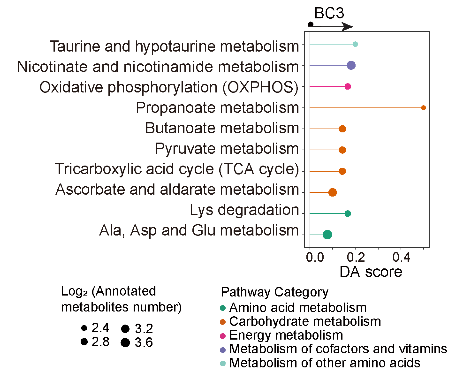
5.12 (S5 I-J) GSEA between BC3 and BC1/2
I. GSEA unveils pathways significantly enriched in BC3, mirroring the findings of the metabolome analyses.
J. GSEA unveils that cholesterol biosynthesis was significantly enriched in BC3.
#------------------------------------------------------------------------------
#  Step 1: KEGG citrate TCA cycle
#------------------------------------------------------------------------------
library(dplyr)
library(ggplot2)

## Load data and set parameters
gene_all <- data.table::fread("result/Figure4/S5H_gene_B.txt") %>%
  as.data.frame()

a <- readLines("raw_data/tca.txt")
gmt <- strsplit(a, "\t")
names(gmt) <- vapply(gmt, function(y) y[1], character(1))
gmt1 <- lapply(gmt, "[", -c(1:2))

a_temp <- gene_all$logFC
names(a_temp) <- gene_all$name

Ranks_all <- sort(a_temp,decreasing =TRUE)
  gseaParam = 0.5
  minSize=5
  ticksSize = 0.2
  Ranks_all = sort(a_temp,decreasing =TRUE)
  fgseaRes_all <- fgsea::fgsea(gmt1, sort(a_temp,decreasing =TRUE),minSize = minSize,nPermSimple=20000,gseaParam=0.5)

  pval <- fgseaRes_all %>%
    dplyr::pull(pval) %>%
    round(3)
  nes <- fgseaRes_all %>%
    dplyr::pull(NES) %>%
    round(3)

  pathway <- gmt1[[1]]

  stats <- Ranks_all
  rnk <- rank(-stats)
  ord <- order(rnk)
  statsAdj <- stats[ord]
  statsAdj <- sign(statsAdj) * (abs(statsAdj)^gseaParam)
  statsAdj <- statsAdj/max(abs(statsAdj))
  pathway <- unname(as.vector(na.omit(match(pathway, names(statsAdj)))))
  pathway <- sort(pathway)
  gseaRes <- fgsea::calcGseaStat(statsAdj, selectedStats = pathway,
                                 returnAllExtremes = TRUE)
  bottoms <- gseaRes$bottoms
  tops <- gseaRes$tops
  n <- length(statsAdj)
  xs <- as.vector(rbind(pathway - 1, pathway))
  ys <- as.vector(rbind(bottoms, tops))
  toPlot <- data.frame(x = c(0, xs, n + 1), y = c(0, ys, 0))
  diff <- (max(tops) - min(bottoms))/8
  x = y = NULL
  ## Visualization
  g1 <- ggplot2::ggplot(toPlot, aes(x = x, y = y)) +
    ggplot2::geom_point(color = "green", size = 0.1) +
    ggplot2::geom_hline(yintercept = 0, colour = "gray") +
    geom_line(color = "green") +
    ggplot2::geom_line(color = "green") +
    theme_bw() +
    ggplot2::theme(panel.grid.minor = ggplot2::element_blank(),
                   axis.text.x=ggplot2::element_blank(),axis.ticks.x=ggplot2::element_blank()) +
    ggplot2::labs(x = NULL, y = "enrichment score",title=)+
    ggplot2::scale_x_continuous(expand = c(0, 0),limits = c(0,length(statsAdj)+1))+
    ggplot2::theme(plot.margin = unit(c(5,5,0,5), "mm"))

  g2 <- ggplot2::ggplot(toPlot, aes(x = x, y = y))+
    ggplot2::geom_segment(data = data.frame(x = pathway),
                          mapping = aes(x = x,
                                        y = -1, xend = x, yend = 1),
                          size = ticksSize,color="red") +
    ggplot2::scale_x_continuous(expand = c(0, 0),
                                limits = c(0,length(statsAdj)+1))+
    theme_bw()+
    ggplot2::theme(panel.grid = element_blank(),
                   axis.text.x=element_blank(),axis.ticks.x=element_blank(),
                   axis.text.y=element_blank(),axis.ticks.y=element_blank())+
    ggplot2::labs(x=NULL,y=NULL)+
    ggplot2::theme(plot.margin = unit(c(0,5,0,5), "mm"))

  dat <- data.frame(name=1:length(statsAdj),value=statsAdj)

  g3 <- ggplot2::ggplot(dat,aes(name,value))+
    ggplot2::geom_bar(stat="identity",fill="gray")+
    ggplot2::theme_bw()+
    ggplot2::theme(panel.grid = element_blank())+
    ggplot2::labs(x=NULL)+
    ggplot2::scale_x_continuous(expand = c(0, 0),limits=c(0,length(statsAdj)+1))+
    ggplot2::theme(plot.margin = unit(c(0,5,5,5), "mm"))

  p1 <- cowplot::plot_grid(plotlist = list(g1,g2,g3),nrow=3,
                           rel_heights = c(1,0.2,0.5),scale=1,
                           align ="v",labels=paste0("TCA Cycle"," pval=",pval,";NES=",nes),label_size = 8)
  ggsave("result/Figure4/S5I_GSEA_B_TCA.pdf",p1,width=4,height = 4)

#------------------------------------------------------------------------------
#  Step 2: Mitochondrial gene expression
#------------------------------------------------------------------------------
library(dplyr)
library(ggplot2)

## Load data and set parameters
gene_all <- data.table::fread("result/Figure4/S5H_gene_B.txt") %>%
  as.data.frame()

a <- readLines("raw_data/MITOCHONDRIAL.txt")
gmt <- strsplit(a, "\t")
names(gmt) <- vapply(gmt, function(y) y[1], character(1))
gmt1 <- lapply(gmt, "[", -c(1:2))

a_temp <- gene_all$logFC
names(a_temp) <- gene_all$name

  Ranks_all <- sort(a_temp,decreasing =TRUE)
  gseaParam = 0.5
  minSize=5
  ticksSize = 0.2
  Ranks_all = sort(a_temp,decreasing =TRUE)
  fgseaRes_all <- fgsea::fgsea(gmt1, sort(a_temp,decreasing =TRUE),minSize = minSize,nPermSimple=20000,gseaParam=0.5)

  pval <- fgseaRes_all %>%
    dplyr::pull(pval) %>%
    round(3)
  nes <- fgseaRes_all %>%
    dplyr::pull(NES) %>%
    round(3)

  pathway <- gmt1[[1]]

  stats <- Ranks_all
  rnk <- rank(-stats)
  ord <- order(rnk)
  statsAdj <- stats[ord]
  statsAdj <- sign(statsAdj) * (abs(statsAdj)^gseaParam)
  statsAdj <- statsAdj/max(abs(statsAdj))
  pathway <- unname(as.vector(na.omit(match(pathway, names(statsAdj)))))
  pathway <- sort(pathway)
  gseaRes <- fgsea::calcGseaStat(statsAdj, selectedStats = pathway,
                                 returnAllExtremes = TRUE)
  bottoms <- gseaRes$bottoms
  tops <- gseaRes$tops
  n <- length(statsAdj)
  xs <- as.vector(rbind(pathway - 1, pathway))
  ys <- as.vector(rbind(bottoms, tops))
  toPlot <- data.frame(x = c(0, xs, n + 1), y = c(0, ys, 0))
  diff <- (max(tops) - min(bottoms))/8
  x = y = NULL
  ## Visualization
  g1 <- ggplot2::ggplot(toPlot, aes(x = x, y = y)) +
    ggplot2::geom_point(color = "green", size = 0.1) +
    ggplot2::geom_hline(yintercept = 0,
                        colour = "gray") + geom_line(color = "green") +
    ggplot2::geom_line(color = "green") + theme_bw() +
    ggplot2::theme(panel.grid.minor = ggplot2::element_blank(),
                   axis.text.x=ggplot2::element_blank(),axis.ticks.x=ggplot2::element_blank()) +
    ggplot2::labs(x = NULL, y = "enrichment score",title=)+
    ggplot2::scale_x_continuous(expand = c(0, 0),limits = c(0,length(statsAdj)+1))+
    ggplot2::theme(plot.margin = unit(c(5,5,0,5), "mm"))

  g2 <- ggplot2::ggplot(toPlot, aes(x = x, y = y))+
    ggplot2::geom_segment(data = data.frame(x = pathway),
                          mapping = aes(x = x,
                                        y = -1, xend = x, yend = 1),
                          size = ticksSize,color="red") +
    ggplot2::scale_x_continuous(expand = c(0, 0),limits = c(0,length(statsAdj)+1))+theme_bw()+
    ggplot2::theme(panel.grid = element_blank(),
                   axis.text.x=element_blank(),axis.ticks.x=element_blank(),
                   axis.text.y=element_blank(),axis.ticks.y=element_blank())+
    ggplot2::labs(x=NULL,y=NULL)+
    ggplot2::theme(plot.margin = unit(c(0,5,0,5), "mm"))

  dat <- data.frame(name=1:length(statsAdj),value=statsAdj)

  g3 <- ggplot2::ggplot(dat,aes(name,value))+
    ggplot2::geom_bar(stat="identity",fill="gray")+
    ggplot2::theme_bw()+
    ggplot2::theme(panel.grid = element_blank())+
    ggplot2::labs(x=NULL)+
    ggplot2::scale_x_continuous(expand = c(0, 0),limits=c(0,length(statsAdj)+1))+
    ggplot2::theme(plot.margin = unit(c(0,5,5,5), "mm"))

  p1 <- cowplot::plot_grid(plotlist = list(g1,g2,g3),nrow=3,
                           rel_heights = c(1,0.2,0.5),scale=1,
                           align ="v",labels=paste0("MITOCHONDRIAL"," pval=",pval,";NES=",nes),label_size = 8)
  ggsave("result/Figure4/S5I_GSEA_B_MITOCHONDRIAL.pdf",p1,width=4,height = 4)

#------------------------------------------------------------------------------
# Step 3: Cholesterol biosynthesis pathway
#------------------------------------------------------------------------------
library(dplyr)
library(ggplot2)

## Load data and set parameters
gene_all <- data.table::fread("result/Figure4/S5H_gene_B.txt") %>%
  as.data.frame()

a <- readLines("raw_data/Cholesterol.txt")
gmt <- strsplit(a, "\t")
names(gmt) <- vapply(gmt, function(y) y[1], character(1))
gmt1 <- lapply(gmt, "[", -c(1:2))

a_temp <- gene_all$logFC
names(a_temp) <- gene_all$name

  Ranks_all <- sort(a_temp,decreasing =TRUE)
  gseaParam = 0.5
  minSize=5
  ticksSize = 0.2
  Ranks_all = sort(a_temp,decreasing =TRUE)
  fgseaRes_all <- fgsea::fgsea(gmt1, sort(a_temp,decreasing =TRUE),minSize = minSize,nPermSimple=20000,gseaParam=0.5)

  pval <- fgseaRes_all %>%
    dplyr::pull(pval) %>%
    round(3)
  nes <- fgseaRes_all %>%
    dplyr::pull(NES) %>%
    round(3)

  pathway <- gmt1[[1]]

  stats <- Ranks_all
  rnk <- rank(-stats)
  ord <- order(rnk)
  statsAdj <- stats[ord]
  statsAdj <- sign(statsAdj) * (abs(statsAdj)^gseaParam)
  statsAdj <- statsAdj/max(abs(statsAdj))
  pathway <- unname(as.vector(na.omit(match(pathway, names(statsAdj)))))
  pathway <- sort(pathway)
  gseaRes <- fgsea::calcGseaStat(statsAdj, selectedStats = pathway,
                                 returnAllExtremes = TRUE)
  bottoms <- gseaRes$bottoms
  tops <- gseaRes$tops
  n <- length(statsAdj)
  xs <- as.vector(rbind(pathway - 1, pathway))
  ys <- as.vector(rbind(bottoms, tops))
  toPlot <- data.frame(x = c(0, xs, n + 1), y = c(0, ys, 0))
  diff <- (max(tops) - min(bottoms))/8
  x = y = NULL
  ## Visualization
  g1 <- ggplot2::ggplot(toPlot, aes(x = x, y = y)) +
    ggplot2::geom_point(color = "green", size = 0.1) +
    ggplot2::geom_hline(yintercept = 0,
                        colour = "gray") + geom_line(color = "green") +
    ggplot2::geom_line(color = "green") + theme_bw() +
    ggplot2::theme(panel.grid.minor = ggplot2::element_blank(),
                   axis.text.x=ggplot2::element_blank(),axis.ticks.x=ggplot2::element_blank()) +
    ggplot2::labs(x = NULL, y = "enrichment score",title=)+
    ggplot2::scale_x_continuous(expand = c(0, 0),limits = c(0,length(statsAdj)+1))+
    ggplot2::theme(plot.margin = unit(c(5,5,0,5), "mm"))

  g2 <- ggplot2::ggplot(toPlot, aes(x = x, y = y))+
    ggplot2::geom_segment(data = data.frame(x = pathway),
                          mapping = aes(x = x,
                                        y = -1, xend = x, yend = 1),
                          size = ticksSize,color="red") +
    ggplot2::scale_x_continuous(expand = c(0, 0),limits = c(0,length(statsAdj)+1))+theme_bw()+
    ggplot2::theme(panel.grid = element_blank(),
                   axis.text.x=element_blank(),axis.ticks.x=element_blank(),
                   axis.text.y=element_blank(),axis.ticks.y=element_blank())+
    ggplot2::labs(x=NULL,y=NULL)+
    ggplot2::theme(plot.margin = unit(c(0,5,0,5), "mm"))

  dat <- data.frame(name=1:length(statsAdj),value=statsAdj)

  g3 <- ggplot2::ggplot(dat,aes(name,value))+
    ggplot2::geom_bar(stat="identity",fill="gray")+
    ggplot2::theme_bw()+
    ggplot2::theme(panel.grid = element_blank())+
    ggplot2::labs(x=NULL)+
    ggplot2::scale_x_continuous(expand = c(0, 0),limits=c(0,length(statsAdj)+1))+
    ggplot2::theme(plot.margin = unit(c(0,5,5,5), "mm"))

  p1 <- cowplot::plot_grid(plotlist = list(g1,g2,g3),nrow=3,
                           rel_heights = c(1,0.2,0.5),scale=1,
                           align ="v",labels=paste0("Cholesterol Biosynthesis"," pval=",pval,";NES=",nes),label_size = 8)
  ggsave("result/Figure4/S5J_GSEA_B_Cholesterol.pdf",p1,width=4,height = 4)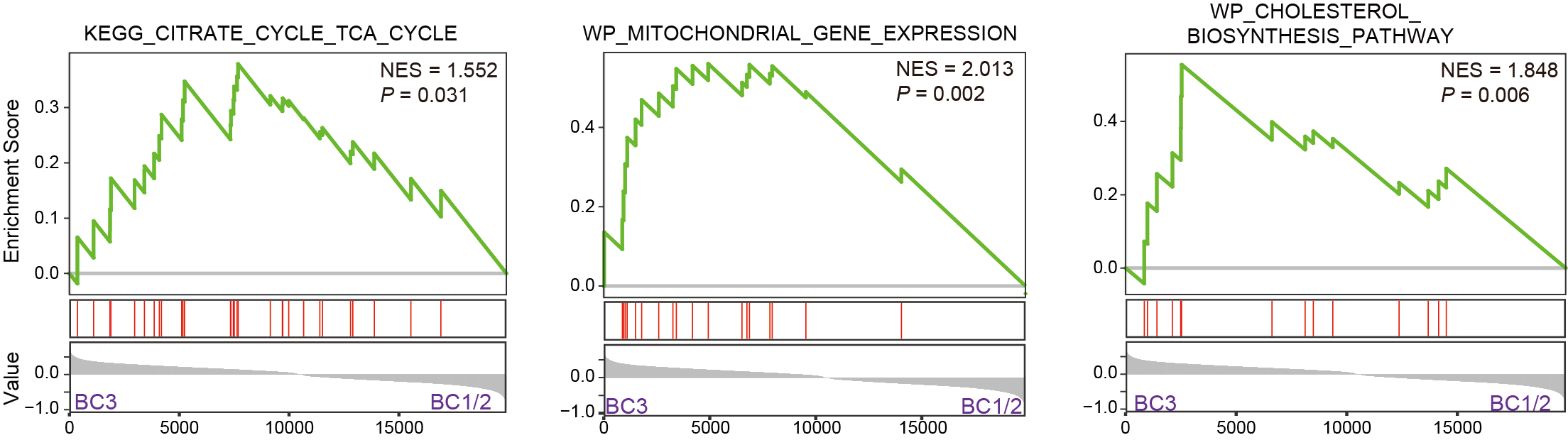
5.13 (S6 A) Clusters of T-ALL
The relative abundance of input metabolites and expression of metabolic genes in the two metabolic clusters: TC1 (N=10) and TC2 (N=14). Each column represents a sample and each row represents a metabolite (upper panel) or gene included (lower panel).
library(dplyr)

sample_info <- data.table::fread("result/Figure4/4F_cluster_T.txt") %>%
  as.data.frame()

metabolite_norm = data.table::fread("result/Figure4/4F_metabolite_norm_T.txt") %>%
  as.data.frame() %>%
  tibble::column_to_rownames("V1")

metgene_norm <- data.table::fread("result/Figure4/4F_metgene_norm_T.txt") %>%
  as.data.frame() %>%
  tibble::column_to_rownames("V1")

top_annotation = HeatmapAnnotation(
  Subtype=sample_info$Clusters,
  col=list(Subtype=c("TC1"="#9BD53F","TC2"="#A6CEE3")),
  show_annotation_name = c(T,T),
  border = c(T,T) ,
  simple_anno_size = unit(4, "mm"),gap = unit(1, "mm"))

col_fun = circlize::colorRamp2(c(-1, 0, 1), c("#00599F", "white", "#D01910"))

p_metabolite <- Heatmap(t(metabolite_norm),height=unit(10,"cm"),
                        name="Metabolite Data",
                        cluster_row_slices = F,clustering_method_rows = "ward.D",
                        clustering_method_columns = "ward.D2",
                        column_split = sample_info$Clusters,
                        col = col_fun,
                        top_annotation =top_annotation,
                        show_column_names = F,show_row_names = F,
                        row_names_gp = gpar(fontsize = 3),
                        column_names_gp = gpar(fontsize = 3))

col_fun = circlize::colorRamp2(c(-1, 0, 1), c("#00599F", "white", "#FF7F00"))

p_gene <- Heatmap(t(metgene_norm),height=unit(10,"cm"),name="Gene Data",
                  cluster_row_slices = F,clustering_method_rows = "ward.D",
                  clustering_method_columns = "ward.D2",
                  column_split = sample_info$Clusters,
                  col = col_fun,
                  show_column_names = F,show_row_names = F,
                  row_names_gp = gpar(fontsize = 3),
                  column_names_gp = gpar(fontsize = 3))

pdf(paste0("result/Figure4/S6A_heatmap_T.pdf"),width=8,height = 10)
p_metabolite %v% p_gene
dev.off()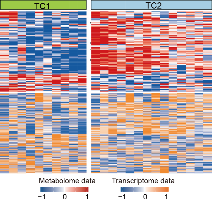
5.14 (S6 E-F) RFS and EFS of TC1/2
The associations of the two metabolic clusters with clinical RFS (E) and EFS (F) outcomes in T-ALL patients. The results suggests TC1 could be of significantly poorer prognosis than TC2.
library(dplyr)
library(survival)
library(ggplot2)

#------------------------------------------------------------------------------
#  Step 1: RFS of TC1/2
#------------------------------------------------------------------------------
survival_new <- readxl::read_excel("raw_data/Meta_Files.xlsx",skip=1) %>%
  as.data.frame() %>%
  dplyr::select(PID,OS_stat,`OS (days)`,"EFS_stat","EFS (days)","RFS_stat","RFS (days)" ) %>%
  dplyr::rename("OS"="OS (days)","EFS"="EFS (days)","RFS"="RFS (days)")

clinical_survival <- data.table::fread(paste0("result/Figure4/4F_cluster_T.txt")) %>%
  as.data.frame() %>%
  dplyr::select(-OS_stat,-OS,-EFS_stat,-EFS,-RFS_stat,-RFS) %>%
  left_join(survival_new,by=c("Pid"="PID"))

surv_object <- Surv(time = clinical_survival$RFS/30, event = clinical_survival$RFS_stat)
fit_cluster <- survfit(surv_object ~ Clusters, data = clinical_survival)
p1 <- survminer::ggsurvplot(fit_cluster, data = clinical_survival,
                            title="RFS",
                palette=c("#9BD53F","#A6CEE3","#EA644C"),
                            tables.theme = theme_void(),risk.table = TRUE,
                            risk.table.fontsize=6,
                            break.time.by = 12,
                            risk.table.y.text = FALSE, tables.height = 0.15,risk.table.col = "black",
                            pval = TRUE,pval.method = F,pval.coord=c(0.5,0.1),pval.size=6,
                            font.tickslab=c(14,"plain","black"),
                            xlab="Time (Months) ",ylab="RFS Survival")

pdf(paste0("result/Figure4/S6E_RFS_T.pdf"),onefile=FALSE)
p1
dev.off()

#------------------------------------------------------------------------------
#  Step 2: EFS
#------------------------------------------------------------------------------
clinical_survival <- data.table::fread(paste0("result/Figure4/4F_cluster_T.txt")) %>%
  as.data.frame()

surv_object <- Surv(time = clinical_survival$EFS/30, event = clinical_survival$EFS_stat)
fit_cluster <- survfit(surv_object ~ Clusters, data = clinical_survival)

p1 <- survminer::ggsurvplot(fit_cluster, data = clinical_survival,
                            title="EFS",
                palette=c("#9BD53F","#A6CEE3","#EA644C"),
                            tables.theme = theme_void(),risk.table = TRUE,
                            risk.table.fontsize=6,
                            break.time.by = 12,
                            risk.table.y.text = FALSE, tables.height = 0.15,risk.table.col = "black",
                            pval = TRUE,pval.method = F,pval.coord=c(0.5,0.1),pval.size=6,
                            font.tickslab=c(14,"plain","black"),
                            xlab="Time (Months) ",ylab="EFS Survival")

pdf(paste0("result/Figure4/S6F_EFS_T.pdf"),onefile=FALSE)
p1
dev.off()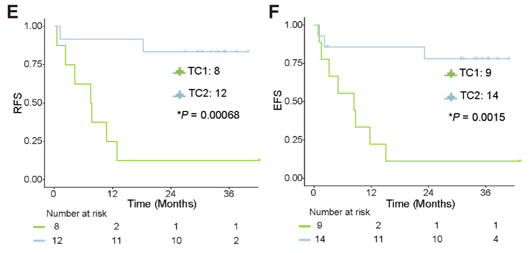
5.15 (S6 H) Multivariate Cox Analysis of TC1/2
The multivariate Cox analysis suggests TC1 may represent an unfavorable group independent of HSCT status. The WBC was stratified by 100×109/L, genetic risk was evaluated according to the NCCN guideline (V 2.2023) including RAS signaling, PTEN and NOTCH1/FBXW7, RAS/PTEN mutation and/or NOTCH1/FBXW7 wildtype were considered as having high risk, otherwise with low risk.
library(dplyr)
library(openxlsx)
library(survival)
library(survminer)

#------------------------------------------------------------------------------
#  Step 1: Load data and set parameters
#------------------------------------------------------------------------------
M_label <- data.table::fread("result/Figure4/4F_cluster_T.txt") %>%
  as.data.frame() %>%
  dplyr::mutate(Clusters=as.factor(Clusters)) %>%
  dplyr::select(Clusters,Pid)

ras <- data.table::fread("raw_data/RAS.txt") %>%
  as.data.frame()  %>%
  dplyr::mutate(name=stringr::str_to_upper(name))

mut <- readxl::read_excel("raw_data/Sample_RNA_190_fusion_mutation_v1130.xlsx") %>%
  dplyr::select(mutation,RNA_id,bianhao) %>%
  tidyr::separate_rows(mutation,sep=";") %>%
  dplyr::mutate(mutation=stringr::str_to_upper(mutation)) %>%
  dplyr::mutate(ras=ifelse(mutation %in% ras$name,"yes","no")) %>%
  dplyr::group_by(RNA_id,bianhao) %>%
  dplyr::summarise(Ras1=paste(ras,collapse = ";"),mutation1=paste(mutation,collapse = ";")) %>%
  dplyr::mutate(ras_new=ifelse(grepl("yes",Ras1),"yes","no"))

genetic <- read.xlsx("raw_data/Sample_RNA_190_fusion_mutation_v1130.xlsx") %>%
  dplyr::select(bianhao,fusion,mutation) %>%
  inner_join(mut,by="bianhao")

names(genetic)

T_gene <- genetic %>%
  dplyr::select(mutation,bianhao,ras_new) %>%
  dplyr::mutate(RAS_PTEN=ifelse(ras_new=="yes","MUT",
                                ifelse(grepl("PTEN",mutation),"MUT","WT"))) %>%
  dplyr::mutate(NOTCH1_FBXW7=ifelse(grepl("NOTCH1",mutation),"MUT",
                                    ifelse(grepl("FBXW7",mutation),"MUT", "WT"))) %>%
  dplyr::mutate(risk=ifelse(RAS_PTEN=="WT"& NOTCH1_FBXW7=="MUT","Low","High")) %>%
  dplyr::select(bianhao,risk) %>%
  dplyr::mutate(Pid=gsub("A","RJ-",bianhao))

##### new survival #####
clinical_survival <- readxl::read_excel("raw_data/Meta_Files.xlsx",skip=1) %>%
  as.data.frame() %>%
  dplyr::rename("OS"="OS (days)","EFS"="EFS (days)","RFS"="RFS (days)","ifHSCT"="HSCT_stat",
         "WBC"="WBC (10⁹/L)","Age"="Age (yrs)","Pid"="PID","RNA_id_raw"="RNA_ID_raw") %>%
  dplyr::select(Pid,RNA_id_raw,Age,Sex,WBC,ifHSCT,OS,OS_stat,EFS,EFS_stat,RFS,RFS_stat,D28_status) %>%
  dplyr::inner_join(M_label,by="Pid") %>%
  dplyr::mutate(WBC_type= ifelse(WBC > 100, "High",
                                 ifelse(WBC <= 100,"Low",WBC))) %>%
  dplyr::mutate(ifHSCT=as.factor(ifHSCT)) %>%
  dplyr::mutate(Age=ifelse(Age>40,"old","young")) %>%
  dplyr::mutate(Age=factor(Age,levels=c("young","old"))) %>%
  dplyr::mutate(Clusters=factor(Clusters)) %>%
  unique() %>%
  dplyr::left_join(T_gene,by="Pid") %>%
  dplyr::mutate(Clusters=factor(Clusters,levels=c("TC2","TC1"))) %>%
  dplyr::mutate(WBC_type=factor(WBC_type,levels=c("Low","High")))

var.names <- c("Clusters","WBC_type","D28_status","ifHSCT","risk")

#-------------------------------------------------------------------------------
#  Step 2: EFS of T-ALL
#-------------------------------------------------------------------------------
f_efs <- as.formula(paste('Surv(EFS, EFS_stat)~',paste(var.names,collapse = "+")))
fit.final <- coxph(f_efs,data=clinical_survival)
p_efs <- ggforest(fit.final,main="EFS Hzard Ratio",cpositions=c(0.02,0.22,0.4),fontsize=0.8,
                  refLabel="reference",noDigits=2,data=clinical_survival)

#-------------------------------------------------------------------------------
#  Step 3: OS of T-ALL
#-------------------------------------------------------------------------------
f_os <- as.formula(paste('Surv(OS, OS_stat)~',paste(var.names,collapse = "+")))
fit.os <- coxph(f_os,data=clinical_survival)
p_os <- ggforest(fit.os,main="OS Hzard Ratio",cpositions=c(0.02,0.22,0.4),fontsize=0.8,
                 refLabel="reference",noDigits=2,data=clinical_survival)
ggsave(p_efs,filename = "result/Figure4/S6H_HR_EFS_T.pdf",width=8,height=4)
ggsave(p_os,filename = "result/Figure4/S6H_HR_OS_T.pdf",width=8,height=4)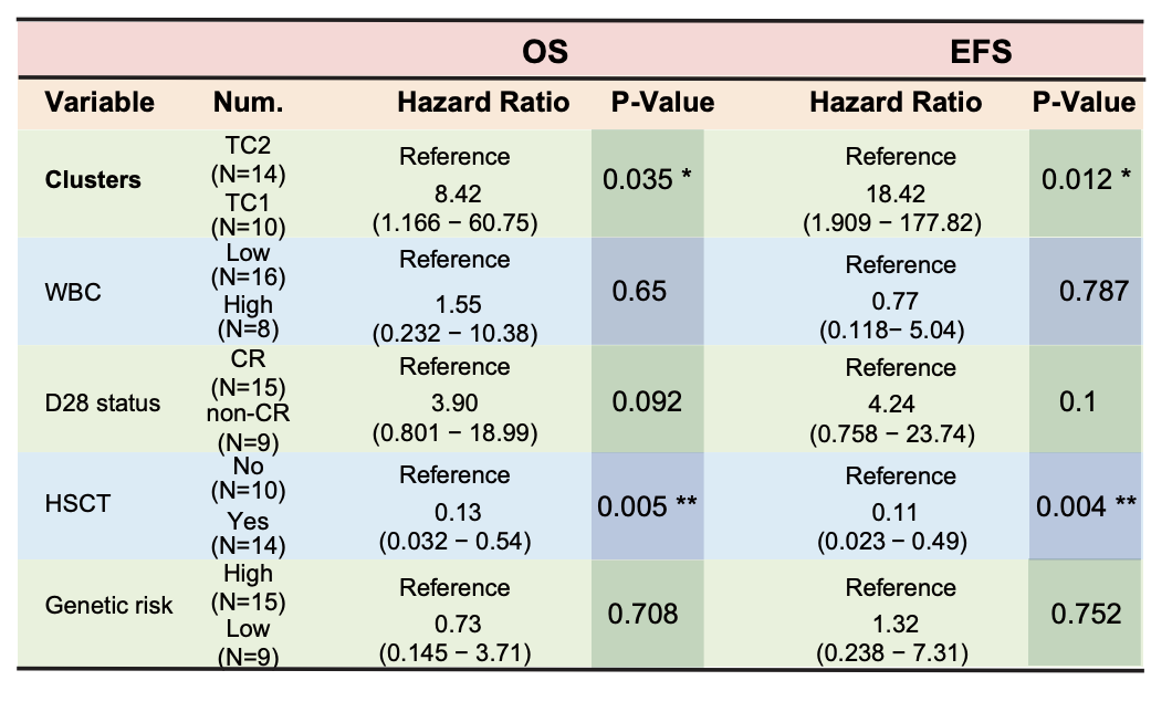
5.16 (S6 I) Waterfall plot of TC1/2
The associations of metabolic clusters with clinical variables and genetic alterations, including major mutations and fusions in T-ALL.
library(dplyr)
library(ComplexHeatmap)

#-------------------------------------------------------------------------------
#  Step 1: Load data and set parameters
#-------------------------------------------------------------------------------

clinical_survival <- readxl::read_excel("raw_data/Meta_Files.xlsx",skip=1) %>%
  as.data.frame() %>%
  dplyr::rename("OS"="OS (days)","EFS"="EFS (days)","RFS"="RFS (days)","ifHSCT"="HSCT_stat",
         "WBC"="WBC (10⁹/L)","Age"="Age (yrs)","Pid"="PID","RNA_id_raw"="RNA_ID_raw") %>%
  dplyr::select(Pid,RNA_id_raw,Age,Sex,WBC,ifHSCT,OS_stat,D28_status,Subtype) %>%
  dplyr::mutate(Age=ifelse(Age < 40,"< 40",">= 40")) %>%
  dplyr::mutate(WBC_type= ifelse(WBC > 100, "> 100",
                                 ifelse(WBC <= 100,"<= 100",NA))) %>%
  dplyr::mutate(Outcome=ifelse(OS_stat==1,"Dead",
                               ifelse(OS_stat==0,"Alive",OS_stat))) %>%
  dplyr::mutate(ifHSCT=ifelse(ifHSCT==0,"no",
                              ifelse(ifHSCT==1,"yes",ifHSCT)))

sample_info <- data.table::fread("result/Figure4/4F_cluster_T.txt") %>%
  as.data.frame() %>%
  dplyr::select(Clusters,Pid) %>%
  dplyr::mutate(bianhao=gsub("RJ-","A",Pid)) %>%
  dplyr::left_join(clinical_survival,by="Pid")

q12 <- c("#1F78B4","#E31A1C","black")
names(q12) <- unique(sample_info$Clusters)

top_annotation = HeatmapAnnotation(
  Subtype=sample_info$Clusters,
  Immunophenotype=sample_info$Subtype,
  ifHSCT=sample_info$ifHSCT,
  WBC=sample_info$WBC_type,
  Outcome=sample_info$Outcome,
  col=list(Subtype=c("TC1"="#9BD53F","TC2"="#A6CEE3"),
           Immunophenotype=c("ETP"="#F9EE35","non_ETP"="#E7317C"),
           ifHSCT=c("yes"="#CAB2D6","no"="gray"),
           WBC=c("> 100"="#FDBF6F","<= 100"="gray"),
           Outcome=c("Dead"="black","Alive"="gray")
  ),
  show_annotation_name = c(T,T),
  border = c(T,T,T,T,T,T) ,
  simple_anno_size = unit(8, "mm"),gap = unit(1.5, "mm")
)

#-------------------------------------------------------------------------------
#  Step 2: Mutations of T-ALL
#-------------------------------------------------------------------------------
mutation_T <- data.table::fread("raw_data/mutation_T_v1114_all.txt") %>%
  as.data.frame() %>%
  dplyr::select(V2,V17,V19) %>%
  dplyr::rename("ID"="V2","Gene.refGene"="V17","ExonicFunc.refGene"="V19") %>%
  dplyr::select(ID,`Gene.refGene`,`ExonicFunc.refGene`) %>%
  dplyr::mutate(`ExonicFunc.refGene`=
                  ifelse(`ExonicFunc.refGene` %in% c("frameshift deletion","frameshift insertion","frameshift substitution"),"Frameshift",
                         ifelse(`ExonicFunc.refGene` %in% c("nonframeshift deletion","nonframeshift insertion","nonframeshift substitution"),"Nonframeshift",
                                ifelse(`ExonicFunc.refGene` %in% ".","Splice",
                                       ifelse(`ExonicFunc.refGene` %in% "nonsynonymous SNV","Missense",
                                              ifelse(`ExonicFunc.refGene`=="startloss","Startloss",
                                                     ifelse(`ExonicFunc.refGene`=="stopgain","Stopgain",
                                                            ifelse(`ExonicFunc.refGene`=="synonymous SNV","Silent",`ExonicFunc.refGene`)))))))) %>%
  unique() %>%
  dplyr::filter(ID %in% sample_info$RNA_id_raw) %>%
  dplyr::mutate(`Gene.refGene` = ifelse(`Gene.refGene` %in% c("IDH1","IDH2"),"IDH1/2",`Gene.refGene`))

mutation <- rbind(mutation_T)

hit_num <- mutation %>%
  dplyr::group_by(ID,`Gene.refGene`) %>%
  dplyr::summarise(n=n()) %>%
  dplyr::filter(n>1)

mutation <- mutation %>%
  dplyr::left_join(hit_num,by=c("ID","Gene.refGene")) %>%
  dplyr::mutate(`ExonicFunc.refGene`=ifelse(!is.na(n),"Multiple",`ExonicFunc.refGene`)) %>%
  dplyr::select(-n) %>%
  unique() %>%
  dplyr::rename("RNA_id"="ID") %>%
  dplyr::filter(RNA_id %in% sample_info$RNA_id_raw)

mutation_gene_filter <- mutation %>%
  dplyr::select(RNA_id,Gene.refGene) %>%
  unique() %>%
  dplyr::group_by(`Gene.refGene`) %>%
  dplyr::summarise(n=n()) %>%
  dplyr::filter(n>0)
mutation_sort <- rev(names(sort(table(mutation %>% filter(`Gene.refGene` %in% mutation_gene_filter$Gene.refGene) %>% pull(Gene.refGene)))))

mutation <- mutation %>%
  dplyr::filter(`Gene.refGene` %in% mutation_gene_filter$Gene.refGene) %>%
  as.data.frame() %>%
  dplyr::distinct(RNA_id,Gene.refGene,.keep_all = T)

sample_info_filter <- sample_info %>%
  dplyr::select(bianhao,RNA_id_raw)

mutation_dcast <- reshape2::dcast(mutation,RNA_id ~ `Gene.refGene`) %>%
  dplyr::right_join(sample_info_filter,by=c("RNA_id"="RNA_id_raw")) %>%
  dplyr::select(-RNA_id) %>%
  tibble::column_to_rownames("bianhao") %>%
  dplyr::select(all_of(mutation_sort))

mutation_dcast[is.na(mutation_dcast)] <- 0
mutation_dcast[mutation_dcast=="Missense"] <- 1
mutation_dcast[mutation_dcast=="Frameshift"] <- 2
mutation_dcast[mutation_dcast=="Nonframeshift"] <- 3
mutation_dcast[mutation_dcast=="Silent"] <- 4
mutation_dcast[mutation_dcast=="Splice"] <- 5
mutation_dcast[mutation_dcast=="Stopgain"] <- 7
mutation_dcast[mutation_dcast=="Multiple"] <- 8

mutation_dcast1 <- mutation_dcast %>%
  dplyr::mutate_if(is.character,as.numeric) %>%
  rowwise() %>%
  dplyr::mutate(NOTCH=sum(NOTCH1)) %>%
  dplyr::mutate(PHF=sum(PTEN,PHF6)) %>%
  dplyr::mutate(RAS=sum(JAK3,JAK1,STAT5A,MTOR,NRAS,KRAS,TCF7,TCF7)) %>%
  dplyr::mutate(Transcript=sum(MED12,RUNX1,ETV6,CNOT3,MED12,GATA3,BCOR)) %>%
  dplyr::mutate(Epigenetic=sum(`IDH1/2`,DNMT3A,KMT2E,SUZ12,SETD1B,SETD2,NCOR2,
                               EP300,KDM6A)) %>%
  dplyr::mutate(Others=sum(CCND3,CTCF,BOD1L1,CCND3,SATB1,OBSCN,DNM2,CIC)) %>%
  dplyr::mutate(NOTCH=ifelse(NOTCH==0,0,9)) %>%
  dplyr::mutate(PHF=ifelse(PHF==0,0,9)) %>%
  dplyr::mutate(RAS=ifelse(RAS==0,0,9)) %>%
  dplyr::mutate(Transcript=ifelse(Transcript==0,0,9)) %>%
  dplyr::mutate(Epigenetic=ifelse(Epigenetic==0,0,9)) %>%
  dplyr::mutate(Others=ifelse(Others==0,0,9)) %>%
  dplyr::select(NOTCH1,NOTCH,
                PHF6,PTEN,PHF,
                JAK3,JAK1,MTOR,NRAS,KRAS,TCF7,TCF7,STAT5A,RAS,
                ETV6,RUNX1,MED12,CNOT3,MED12,GATA3,BCOR,Transcript,
                DNMT3A,SUZ12,SETD1B,`IDH1/2`,KMT2E,NCOR2,EP300,KDM6A,
                Epigenetic,
                CTCF,CCND3,CCND3,SATB1,OBSCN,DNM2,CIC,BOD1L1,Others) %>%
  as.data.frame()


rownames(mutation_dcast1) <- rownames(mutation_dcast)
mutation_dcast <- mutation_dcast1

mutation_dcast_temp <- mutation_dcast
mutation_dcast_temp[mutation_dcast_temp!=0] <- 1
num=colSums(mutation_dcast_temp)
names(mutation_dcast) <- paste0(names(mutation_dcast)," (n=",num,")")

d_mutation <- t(mutation_dcast) %>%
  as.data.frame() %>%
  dplyr::select(sample_info$bianhao)

mutation_annotation <- Heatmap(d_mutation,height=unit(15,"cm"),rect_gp = gpar(col = "gray", lwd = 2),
                               col=c("#EEEEEE","#3987CC","#DB3D3D","#663FFB","#FF7F0E","#CC66FF","#8B564C","#339933","blue"),
                               cluster_columns = F,cluster_rows = F,border = TRUE,column_title = NULL,
                               column_split =sample_info$Clusters,
                               show_column_names = TRUE,
                               top_annotation=top_annotation,
                               row_names_gp = gpar(fontsize = 8),column_names_gp=gpar(fontsize=6))

#-------------------------------------------------------------------------------
#  Step 3: Fusions of T-ALL
#-------------------------------------------------------------------------------
fusion_T <- readxl::read_excel("raw_data/fusion_T_v0803.xlsx",skip=1) %>%
  as.data.frame() %>%
  dplyr::filter(RNA_id %in% sample_info$RNA_id_raw) %>%
  dplyr::select(RNA_id,final_check) %>%
  dplyr::left_join(sample_info,by=c("RNA_id"="RNA_id_raw")) %>%
  dplyr::select(RNA_id,final_check) %>%
  dplyr::filter(!is.na(final_check))

fusion <- rbind(fusion_T)

clinical_fusion_dcast <- reshape2::dcast(fusion,RNA_id ~ final_check) %>%
  dplyr::right_join(sample_info_filter,by=c("RNA_id"="RNA_id_raw")) %>%
  tibble::column_to_rownames("bianhao") %>%
  dplyr::select(-RNA_id)

clinical_fusion_dcast[is.na(clinical_fusion_dcast)] <- 0
clinical_fusion_dcast[clinical_fusion_dcast != 0] <- 1

d_fusion <- t(clinical_fusion_dcast) %>%
  as.data.frame() %>%
  dplyr::select(sample_info$bianhao) %>%
  tibble::rownames_to_column(var="fusion") %>%
  dplyr::arrange(match(fusion,c("SET-NUP214","MLLT10 rearrangement","NUP98","STIL-TAL1",
                                "KMT2A rearrangement","other"))) %>%
  tibble::column_to_rownames("fusion")

fusion_annotation <- Heatmap(d_fusion,rect_gp = gpar(col = "gray", lwd = 2),
                             col=c("#EEEEEE","#444444"),
                             height=unit(2,"cm"),border = TRUE,
                             column_split =sample_info$Clusters,
                             cluster_columns = F,cluster_rows = F,column_title = NULL,
                             row_names_gp = gpar(fontsize = 8),column_names_gp=gpar(fontsize=6))

#-------------------------------------------------------------------------------
#  Step 4: Visualization
#-------------------------------------------------------------------------------
pdf(paste0("result/Figure4/S6I_oncoplot_T.pdf"),width=7,height = 10)
mutation_annotation %v% fusion_annotation
dev.off()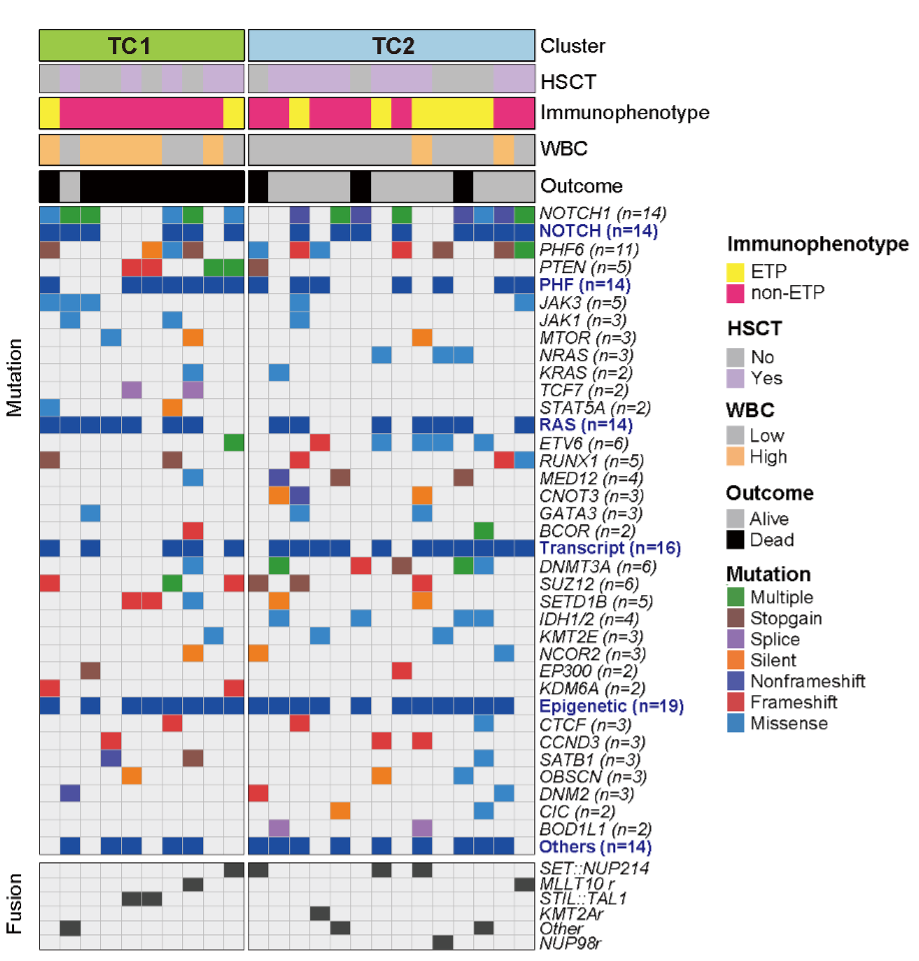
5.17 (S6 J) DA score of TC1/2
DA-score demonstrates that most of the metabolic pathways are upregulated in the relatively favorable TC2 cluster.
library(ggplot2)
library(MNet)
library(dplyr)

#------------------------------------------------------------------------------
#  Step 1: DA-score of gene_T
#------------------------------------------------------------------------------
cluster <- data.table::fread("result/Figure4/4F_cluster_T.txt") %>%
  as.data.frame()
dat <- data.table::fread("raw_data/cell_dat_final_reuslt_v0329.txt") %>%
  dplyr::select(label,all_of(cluster$METc_BM_D0_ID)) %>%
  tibble::column_to_rownames("label")
group <- cluster$Clusters
table(group)
group[which(group== "TC1")] <- "tumor"
group[which(group== "TC2")] <- "normal"
metabolite_all <- mlimma(log1p(dat),group)
write.table(metabolite_all,"result/Figure4/S6J_metabolite_T.txt",quote=F,row.names=F,sep="\t")

dd <- metabolite_all %>%
  dplyr::mutate(Condition=ifelse(logFC>0 & P.Value < 0.05,"Up",
                          ifelse(logFC < 0 & P.Value < 0.05,"Down","normal")))

cluster <- data.table::fread("result/Figure4/4F_cluster_T.txt") %>%
  as.data.frame()

dat <- readRDS("raw_data/20231113_RNA_ALL_VST_coding.rds") %>%
  as.data.frame() %>%
  dplyr::select(all_of(cluster$RNA_id_raw))
group <- cluster$Clusters

group[which(group== "TC1")] <- "tumor"
group[which(group== "TC2")] <- "normal"

gene_all <- mlimma(dat,group)

write.table(gene_all,"result/Figure4/S6J_gene_T.txt",quote=F,row.names=F,sep="\t")

dat <- data.table::fread("result/Figure4/S6J_gene_T.txt")

dat_increase <- dat %>%
  dplyr::filter(logFC > 0) %>%
  dplyr::filter(P.Value < 0.05)
dat_decrease <- dat %>%
  dplyr::filter(logFC < 0) %>%
  dplyr::filter(P.Value < 0.05)

DA_result <- DAscore(dat_increase$name,dat_decrease$name,dat$name,min_measured_num = 10,out="gene")
DAscore_gene_T <- DA_result$result

#------------------------------------------------------------------------------
#  Step 2: DA-score of metabolite_T
#------------------------------------------------------------------------------
kegg_id <- readxl::read_excel("raw_data/cell_metabolite_info_all_v1109.xlsx") %>%
  as.data.frame() %>%
  dplyr::select(refmet_name,KEGG) %>%
  tidyr::separate_rows(KEGG,sep=";") %>%
  dplyr::filter(KEGG!="NA") %>%
  dplyr::filter(KEGG != "None") %>%
  as.data.frame()

dat <- data.table::fread("result/Figure4/S6J_metabolite_T.txt") %>%
  dplyr::arrange(desc(logFC)) %>%
  dplyr::inner_join(kegg_id,by=c("name"="refmet_name")) %>%
  dplyr::distinct(KEGG,.keep_all = TRUE)

dat_increase <- dat %>%
  dplyr::filter(logFC > 0) %>%
  dplyr::filter(P.Value < 0.05)
dat_decrease <- dat %>%
  dplyr::filter(logFC < 0) %>%
  dplyr::filter(P.Value < 0.05)

DA_result <- DAscore(dat_increase$KEGG,dat_decrease$KEGG,dat$KEGG,min_measured_num = 3,out="metabolite")
write.table(DA_result$result,"result/Figure4/S6J_DAscore_metabolite_T.txt",quote=F,row.names=F,sep="\t")

#------------------------------------------------------------------------------
#  Step 3: DA-score of gene+metabolite_T
#------------------------------------------------------------------------------
gene <- DAscore_gene_T %>%
  as.data.frame() %>%
  dplyr::filter(Measured_members_num >= 10) %>%
  dplyr::filter(abs(DA_score) > 0.05)

metabolite <- data.table::fread("result/Figure4/S6J_DAscore_metabolite_T.txt") %>%
  as.data.frame() %>%
  dplyr::filter(Measured_members_num >= 3) %>%
  dplyr::filter(DA_score != 0)

all_1 <- gene %>%
  dplyr::inner_join(metabolite,by="Pathway") %>%
  dplyr::filter(DA_score.x >0 & DA_score.y >0)

all_2 <- gene %>%
  dplyr::inner_join(metabolite,by="Pathway") %>%
  dplyr::filter(DA_score.x < 0 & DA_score.y < 0)

path <- c(all_1$Pathway,all_2$Pathway)

colp <- c("Amino acid metabolism" ="#1B9E77",
          "Carbohydrate metabolism"="#D95F02",
          "Glycan biosynthesis and metabolism"="#1F78B4",
          "Metabolism of cofactors and vitamins"="#7570B3",
          "Metabolism of terpenoids and polyketides"="#BC80BD",
          "Metabolism of other amino acids"="#8DD3C7",
          "Energy metabolism"="#E7298A",
          "Lipid metabolism"="#66A61E",
          "Nucleotide metabolism"="#E6AB02",
          "Biosynthesis of other secondary metabolites"="#A6761D",
          "Xenobiotics biodegradation and metabolism"="#666666")

metabolite_filter <- metabolite %>%
  dplyr::filter(Pathway %in% path) %>%
  dplyr::filter(Measured_members_num >= 3) %>%
  dplyr::filter(abs(DA_score) > 0.05) %>%
  dplyr::arrange(`Pathway Category`) %>%
  dplyr::mutate(Pathway=factor(Pathway,levels = Pathway))

colp <- c("Amino acid metabolism" ="#1B9E77",
          "Carbohydrate metabolism"="#D95F02",
          "Glycan biosynthesis and metabolism"="#1F78B4",
          "Metabolism of cofactors and vitamins"="#7570B3",
          "Metabolism of terpenoids and polyketides"="#BC80BD",
          "Metabolism of other amino acids"="#8DD3C7",
          "Energy metabolism"="#E7298A",
          "Lipid metabolism"="#66A61E",
          "Nucleotide metabolism"="#E6AB02",
          "Biosynthesis of other secondary metabolites"="#A6761D",
          "Xenobiotics biodegradation and metabolism"="#666666")

p <- ggplot(metabolite_filter)+
  geom_point(aes(x=Pathway,y=DA_score,size=log2(Measured_members_num),color=`Pathway Category`))+
  geom_pointrange(aes(x=Pathway,y=DA_score,ymin=0,ymax=DA_score,color=`Pathway Category`))+
  scale_color_manual(values=colp)+
  coord_flip()+
  xlab(NULL)+
  theme_bw()

ggsave("result/Figure4/S6J_DAscore_metabolite_T_filter.pdf",p,width=8,height = 3.5)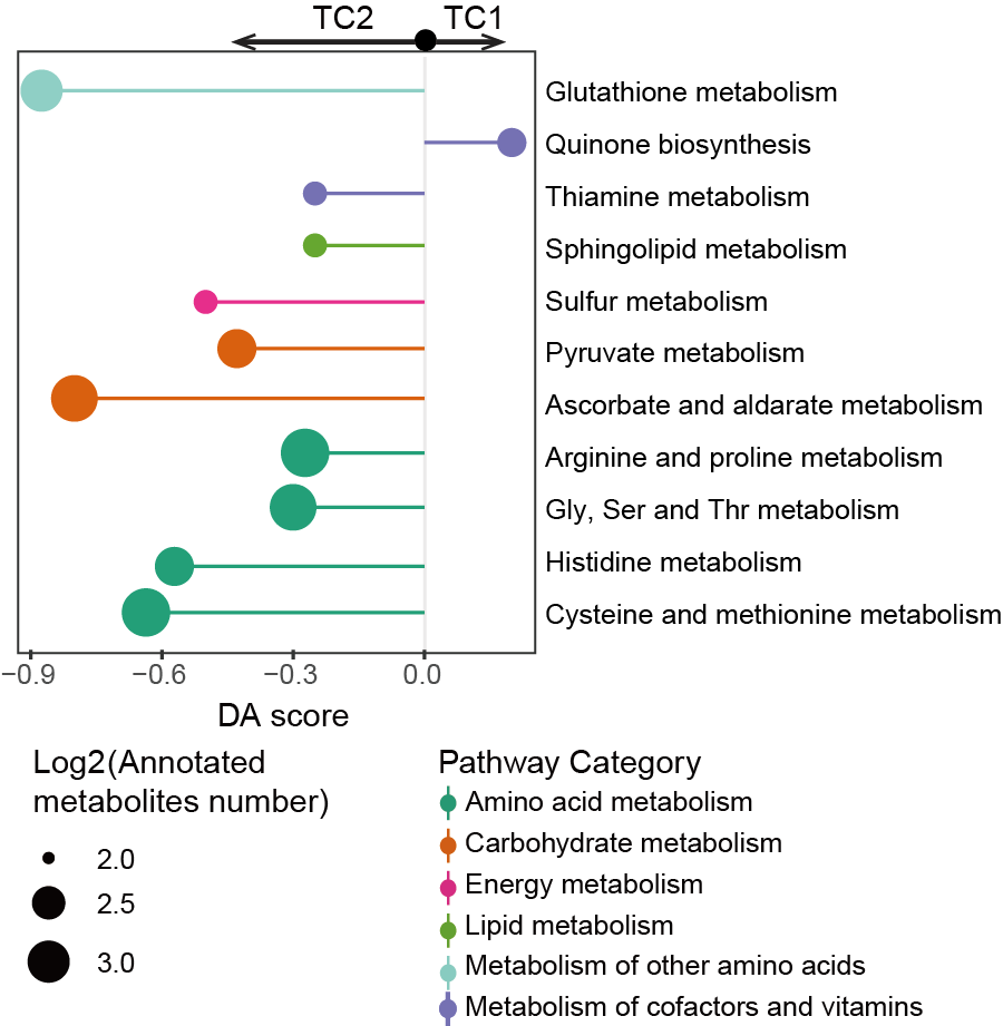
5.18 (S6 K-L) GSEA between TC1 and TC2
The GSEA reveals that the TC1 cluster, associated with poorer prognosis, exhibits suppression in OXPHOS and enrichment in histone modifications.
#------------------------------------------------------------------------------
#  Step 1: Oxidative phosphorylation
#------------------------------------------------------------------------------
library(dplyr)
library(ggplot2)

## Load data
gene_all <- data.table::fread("result/Figure4/S6J_gene_T.txt") %>%
  as.data.frame()

a <- readLines("raw_data/OXIDATIVE.txt")
gmt <- strsplit(a, "\t")
names(gmt) <- vapply(gmt, function(y) y[1], character(1))
gmt1 <- lapply(gmt, "[", -c(1:2))

a_temp <- gene_all$logFC
names(a_temp) <- gene_all$name
  ##GSEA
  Ranks_all <- sort(a_temp,decreasing =TRUE)
  gseaParam = 1
  minSize=5
  ticksSize = 0.2
  Ranks_all = sort(a_temp,decreasing =TRUE)
  fgseaRes_all <- fgsea::fgsea(gmt1, sort(a_temp,decreasing =TRUE),minSize = minSize,nPermSimple=20000,gseaParam=1)

  pval <- fgseaRes_all %>%
    dplyr::pull(pval) %>%
    round(3)
  nes <- fgseaRes_all %>%
    dplyr::pull(NES) %>%
    round(3)

  pathway <- gmt1[[1]]

  stats <- Ranks_all
  rnk <- rank(-stats)
  ord <- order(rnk)
  statsAdj <- stats[ord]
  statsAdj <- sign(statsAdj) * (abs(statsAdj)^gseaParam)
  statsAdj <- statsAdj/max(abs(statsAdj))
  pathway <- unname(as.vector(na.omit(match(pathway, names(statsAdj)))))
  pathway <- sort(pathway)
  gseaRes <- fgsea::calcGseaStat(statsAdj, selectedStats = pathway,
                                 returnAllExtremes = TRUE)
  bottoms <- gseaRes$bottoms
  tops <- gseaRes$tops
  n <- length(statsAdj)
  xs <- as.vector(rbind(pathway - 1, pathway))
  ys <- as.vector(rbind(bottoms, tops))
  toPlot <- data.frame(x = c(0, xs, n + 1), y = c(0, ys, 0))
  diff <- (max(tops) - min(bottoms))/8
  x = y = NULL
  g1 <- ggplot2::ggplot(toPlot, aes(x = x, y = y)) +
    ggplot2::geom_point(color = "green", size = 0.1) +
    ggplot2::geom_hline(yintercept = 0,
                        colour = "gray") + geom_line(color = "green") +
    ggplot2::geom_line(color = "green") + theme_bw() +
    ggplot2::theme(panel.grid.minor = ggplot2::element_blank(),
                   axis.text.x=ggplot2::element_blank(),axis.ticks.x=ggplot2::element_blank()) +
    ggplot2::labs(x = NULL, y = "enrichment score",title=)+
    ggplot2::scale_x_continuous(expand = c(0, 0),limits = c(0,length(statsAdj)+1))+
    ggplot2::theme(plot.margin = unit(c(5,5,0,5), "mm"))

  g2 <- ggplot2::ggplot(toPlot, aes(x = x, y = y))+
    ggplot2::geom_segment(data = data.frame(x = pathway),
                          mapping = aes(x = x,
                                        y = -1, xend = x, yend = 1),
                          size = ticksSize,color="red") +
    ggplot2::scale_x_continuous(expand = c(0, 0),limits = c(0,length(statsAdj)+1))+theme_bw()+
    ggplot2::theme(panel.grid = element_blank(),
                   axis.text.x=element_blank(),axis.ticks.x=element_blank(),
                   axis.text.y=element_blank(),axis.ticks.y=element_blank())+
    ggplot2::labs(x=NULL,y=NULL)+
    ggplot2::theme(plot.margin = unit(c(0,5,0,5), "mm"))

  dat <- data.frame(name=1:length(statsAdj),value=statsAdj)

  g3 <- ggplot2::ggplot(dat,aes(name,value))+
    ggplot2::geom_bar(stat="identity",fill="gray")+
    ggplot2::theme_bw()+
    ggplot2::theme(panel.grid = element_blank())+
    ggplot2::labs(x=NULL)+
    ggplot2::scale_x_continuous(expand = c(0, 0),limits=c(0,length(statsAdj)+1))+
    ggplot2::theme(plot.margin = unit(c(0,5,5,5), "mm"))

  p1 <- cowplot::plot_grid(plotlist = list(g1,g2,g3),nrow=3,
                           rel_heights = c(1,0.2,0.5),scale=1,
                           align ="v",labels=paste0("OXIDATIVE_PHOSPHORYLATION"," pval=",pval,";NES=",nes),label_size = 8)
  ggsave("result/Figure4/S6K_GSEA_T_OXIDATIVE.pdf",p1,width=5,height = 5)

#------------------------------------------------------------------------------
#  Step 2: Histone modifications
#------------------------------------------------------------------------------
## Load data
gene_all <- data.table::fread("result/Figure4/S6J_gene_T.txt") %>%
  as.data.frame()

a <- readLines("raw_data/histone.txt")
gmt <- strsplit(a, "\t")
names(gmt) <- vapply(gmt, function(y) y[1], character(1))
gmt1 <- lapply(gmt, "[", -c(1:2))

a_temp <- gene_all$logFC
names(a_temp) <- gene_all$name

##GSEA
  Ranks_all <- sort(a_temp,decreasing =TRUE)
  gseaParam = 1
  minSize=5
  ticksSize = 0.2
  Ranks_all = sort(a_temp,decreasing =TRUE)
  fgseaRes_all <- fgsea::fgsea(gmt1, sort(a_temp,decreasing =TRUE),minSize = minSize,nPermSimple=20000,gseaParam=0.5)

  pval <- fgseaRes_all %>%
    dplyr::pull(pval) %>%
    round(3)
  nes <- fgseaRes_all %>%
    dplyr::pull(NES) %>%
    round(3)

  pathway <- gmt1[[1]]

  stats <- Ranks_all
  rnk <- rank(-stats)
  ord <- order(rnk)
  statsAdj <- stats[ord]
  statsAdj <- sign(statsAdj) * (abs(statsAdj)^gseaParam)
  statsAdj <- statsAdj/max(abs(statsAdj))
  pathway <- unname(as.vector(na.omit(match(pathway, names(statsAdj)))))
  pathway <- sort(pathway)
  gseaRes <- fgsea::calcGseaStat(statsAdj, selectedStats = pathway,
                                 returnAllExtremes = TRUE)
  bottoms <- gseaRes$bottoms
  tops <- gseaRes$tops
  n <- length(statsAdj)
  xs <- as.vector(rbind(pathway - 1, pathway))
  ys <- as.vector(rbind(bottoms, tops))
  toPlot <- data.frame(x = c(0, xs, n + 1), y = c(0, ys, 0))
  diff <- (max(tops) - min(bottoms))/8
  x = y = NULL
  g1 <- ggplot2::ggplot(toPlot, aes(x = x, y = y)) +
    ggplot2::geom_point(color = "green", size = 0.1) +
    ggplot2::geom_hline(yintercept = 0,
                        colour = "gray") + geom_line(color = "green") +
    ggplot2::geom_line(color = "green") + theme_bw() +
    ggplot2::theme(panel.grid.minor = ggplot2::element_blank(),
                   axis.text.x=ggplot2::element_blank(),axis.ticks.x=ggplot2::element_blank()) +
    ggplot2::labs(x = NULL, y = "enrichment score",title=)+
    ggplot2::scale_x_continuous(expand = c(0, 0),limits = c(0,length(statsAdj)+1))+
    ggplot2::theme(plot.margin = unit(c(5,5,0,5), "mm"))

  g2 <- ggplot2::ggplot(toPlot, aes(x = x, y = y))+
    ggplot2::geom_segment(data = data.frame(x = pathway),
                          mapping = aes(x = x,
                                        y = -1, xend = x, yend = 1),
                          size = ticksSize,color="red") +
    ggplot2::scale_x_continuous(expand = c(0, 0),limits = c(0,length(statsAdj)+1))+theme_bw()+
    ggplot2::theme(panel.grid = element_blank(),
                   axis.text.x=element_blank(),axis.ticks.x=element_blank(),
                   axis.text.y=element_blank(),axis.ticks.y=element_blank())+
    ggplot2::labs(x=NULL,y=NULL)+
    ggplot2::theme(plot.margin = unit(c(0,5,0,5), "mm"))

  dat <- data.frame(name=1:length(statsAdj),value=statsAdj)

  g3 <- ggplot2::ggplot(dat,aes(name,value))+
    ggplot2::geom_bar(stat="identity",fill="gray")+
    ggplot2::theme_bw()+
    ggplot2::theme(panel.grid = element_blank())+
    ggplot2::labs(x=NULL)+
    ggplot2::scale_x_continuous(expand = c(0, 0),limits=c(0,length(statsAdj)+1))+
    ggplot2::theme(plot.margin = unit(c(0,5,5,5), "mm"))

  p1 <- cowplot::plot_grid(plotlist = list(g1,g2,g3),nrow=3,
                           rel_heights = c(1,0.2,0.5),scale=1,
                           align ="v",labels=paste0("histone"," pval=",pval,";NES=",nes),label_size = 8)
  ggsave("result/Figure4/S6L_GSEA_T_histone.pdf",p1,width=4,height = 4)